The hardware and bandwidth for this mirror is donated by dogado GmbH, the Webhosting and Full Service-Cloud Provider. Check out our Wordpress Tutorial.
If you wish to report a bug, or if you are interested in having us mirror your free-software or open-source project, please feel free to contact us at mirror[@]dogado.de.

xsdm

xsdm is an R package that integrates concepts of stochastic demography into species distribution modelling (SDM). Instead of treating environmental conditions as a static snapshot, xsdm uses multi-year environmental time-series together with species presence/absence records to:

Reconstruct a species’ fundamental ecological niche via maximum-likelihood estimation.
Account for inter-annual climate variability when estimating niche breadth and position.
Project the species’ potential geographic range under current or future climate scenarios.

The statistical underpinning is described in:

Berti, E., Robles Fernández, A.L., Rosenbaum, B., Peterson, T.A., Soberón, J., & Reuman, D.C. (2025). The impacts of climate variability on the niche concept and distributions of species. bioRxiv. https://doi.org/10.1101/2024.10.30.621023

Installation

CRAN

install.packages("xsdm")

Development version

Install the latest version directly from GitHub:

# install.packages("remotes")
remotes::install_github("xsdm-project/xsdm-devel")

xsdm requires R ≥ 4.1 and links to C++ via Rcpp/RcppParallel, so a working compiler (e.g. Rtools on Windows, Xcode CLT on macOS) is needed.

Full end-to-end workflow

1 · Load and prepare environmental time series

xsdm expects bioclimatic time-series rasters — one SpatRaster per variable with each layer representing one year (or time step). The built-in data cover southern New Mexico, USA, over 39 years (1980–2018) using CHELSA v2.1 bio1 (mean annual temperature) and bio12 (annual precipitation).

library(xsdm)
library(terra)

bio_1 <- terra::unwrap(example_1$bio01)
bio_1 <- bio_1 / 100

bio_12 <- terra::unwrap(example_1$bio12)
bio_12 <- bio_12 / 100

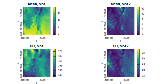
Take a look at the temporal means and standard deviations of the environmental variables:

m_bio_1 <- terra::app(bio_1, mean)
m_bio_12 <- terra::app(bio_12, mean)
sd_bio_1 <- terra::app(bio_1, sd)
sd_bio_12 <- terra::app(bio_12, sd)
par(mfrow = c(2, 2), mar = c(3, 3, 2, 4))
terra::plot(m_bio_1, main = "Mean, bio1", xlab = "x", ylab = "y")
terra::plot(m_bio_12, main = "Mean, bio12", xlab = "x", ylab = "y")
terra::plot(sd_bio_1, main = "SD, bio1", xlab = "x", ylab = "y")
terra::plot(sd_bio_12, main = "SD, bio12", xlab = "x", ylab = "y")

plot of chunk plot-env

2 · Species occurrence data

Load the occurrence data and visualize detections and non-detections on top of the mean temperature map:

d <- example_1$occ_df
pts_0 <- terra::vect(d[d$presence == 0, ], geom = c("lon", "lat"),
                     crs = terra::crs(m_bio_1))
#> Error:
#> ! unable to find an inherited method for function 'vect' for signature 'x = "tbl_df"'
pts_1 <- terra::vect(d[d$presence == 1, ], geom = c("lon", "lat"),
                     crs = terra::crs(m_bio_1))
#> Error:
#> ! unable to find an inherited method for function 'vect' for signature 'x = "tbl_df"'
par(mfrow = c(1, 2), mar = c(3, 3, 2, 4))
terra::plot(m_bio_1, main = "Non-detections", xlab = "x", ylab = "y")
terra::plot(pts_0, add = TRUE, col = "black", pch = 20, cex = 0.2)
#> Error in `h()`:
#> ! error in evaluating the argument 'x' in selecting a method for function 'plot': object 'pts_0' not found
terra::plot(m_bio_1, main = "Detections", xlab = "x", ylab = "y")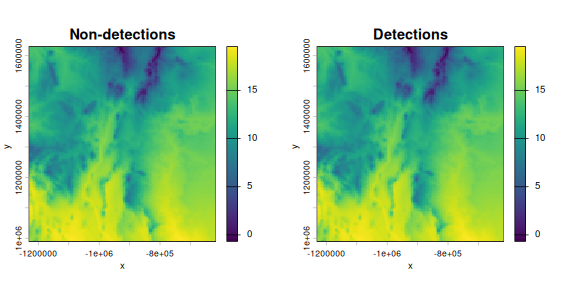

plot of chunk plot-occ

terra::plot(pts_1, add = TRUE, col = "red", pch = 20, cex = 0.2)
#> Error in `h()`:
#> ! error in evaluating the argument 'x' in selecting a method for function 'plot': object 'pts_1' not found

3 · Build the environmental data array

env_data_array() extracts and stacks environmental values at the locations given in a presence/absence data frame, returning a 3-D array (locations × time × variables).

env_data <- list(bio_1 = bio_1, bio_12 = bio_12)
env_dat <- env_data_array(env_data, occ = d)
dim(env_dat)
#> [1] 4000   39    2
occ <- d$presence

4 · Fit the model

optimize_likelihood() runs multiple optimizations from Latin-hypercube starting points and returns every solution sorted by decreasing log-likelihood:

result <- optimize_likelihood(
  env_dat    = env_dat,
  occ        = occ,
  num_starts = 20L,
  parallel   = FALSE,
  verbose    = FALSE
)

head(result$solutions[, c("start_id", "loglik", "convergence")])
#>   start_id    loglik convergence
#> 1       19 -1009.447           4
#> 2        4 -1009.447           4
#> 3       20 -1009.447           4
#> 4       11 -1009.447           4
#> 5        5 -1009.447           4
#> 6        8 -1009.447           4
result$best$loglik
#> [1] -1009.447

5 · Interpret the fitted parameters

Convert the best math-scale parameter vector to the biologically interpretable scale and plot the inferred log growth–environment function:

best_bio <- math_to_bio(result$best$par)

par(mfrow = c(1, 2))
interpret_parameters(
  best_bio,
  plot_indices = c(1, 2),
  env_dat      = env_dat,
  occ          = occ
)

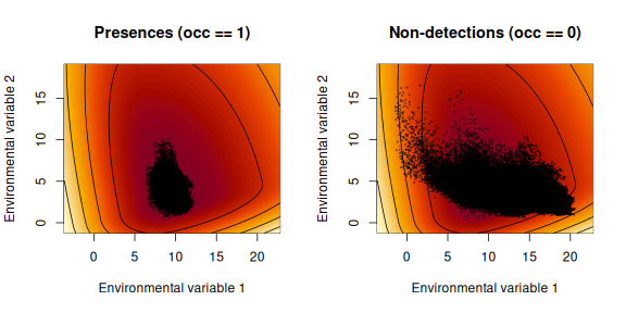
plot of chunk interpret

6 · Habitat suitability map

Use the fitted parameters to project a habitat suitability map over the full raster extent:

hab_suit <- habitat_suitability(
  param_list = best_bio,
  env_list   = env_data
)
terra::plot(hab_suit, main = "Habitat suitability", xlab = "x", ylab = "y")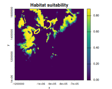

plot of chunk hab-suit

Key functions

Function	Purpose
`env_data_array()`	Build a `(locations × time × variables)` array from raster time series and an occurrence table
`optimize_likelihood()`	Multi-start MLE fitting; returns solutions sorted by log-likelihood
`loglik_math()`	Evaluate the log-likelihood at any math-scale parameter vector
`math_to_bio()`	Convert math-scale vector → biological-scale parameter list
`bio_to_math()`	Convert biological-scale parameter list → math-scale vector
`start_parms()`	Generate Latin-hypercube starting points from presence-only data
`profile_likelihood()`	Profile one parameter while re-optimising over the rest
`habitat_suitability()`	Produce a spatial probability-of-detection map
`interpret_parameters()`	Diagnostic plots of the niche shape
`dist_between_params()`	Distance between two parameter sets (Hungarian algorithm, equivalence-class aware)

For developers and contributors

Install from source

# Clone the repository and install locally
install.packages("devtools")
devtools::install_github("xsdm-project/xsdm-devel")

Reporting issues

Please file bugs and feature requests on the GitHub issue tracker. When reporting a bug, include the output of sessionInfo() and a minimal reproducible example.

Citation

If you use xsdm in published work, please cite:

Berti, E., Robles Fernández, A.L., Rosenbaum, B., Peterson, T.A.,
Soberón, J., & Reuman, D.C. (2025). The impacts of climate variability
on the niche concept and distributions of species. bioRxiv.
https://doi.org/10.1101/2024.10.30.621023

BibTeX:

@article{bertiXSDM1,
  title  = {The impacts of climate variability on the niche concept and
            distributions of species},
  author = {Berti, E. and Fern\'{a}ndez, ALR and Rosenbaum, B and
            Peterson, TA and Sober\'{o}n, J and Reuman, DC},
  journal = {bioRxiv},
  doi    = {10.1101/2024.10.30.621023},
  year   = {2025},
  url    = {https://doi.org/10.1101/2024.10.30.621023}
}

License

xsdm is released under the GNU Affero General Public License, version 3 (AGPL-3.0) or any later version.

These binaries (installable software) and packages are in development.
They may not be fully stable and should be used with caution. We make no claims about them.
Health stats visible at Monitor.