
The hardware and bandwidth for this mirror is donated by dogado GmbH, the Webhosting and Full Service-Cloud Provider. Check out our Wordpress Tutorial.
If you wish to report a bug, or if you are interested in having us mirror your free-software or open-source project, please feel free to contact us at mirror[@]dogado.de.
![]()
![]()
The weird package contains functions and data used in the book That’s Weird: Anomaly Detection Using R by Rob J Hyndman. It also loads several packages needed to do the analysis described in the book.
You can install the stable version from CRAN with:
install.packages("weird")You can install the development version of weird from GitHub with:
# install.packages("pak")
pak::pak("robjhyndman/weird")library(weird) will also load the following
packages:
When you load the weird package, you get a condensed summary of conflicts with other packages you have previously loaded:
library(weird)
#> ── Attaching packages ─────────────────────────────────────────── weird 2.0.0.9000 ──
#> ✔ dplyr          1.2.1     ✔ distributional 0.7.0
#> ✔ ggplot2        4.0.3
#> ── Conflicts ───────────────────────────────────────────────────── weird_conflicts ──
#> ✖ dplyr::filter() masks stats::filter()
#> ✖ dplyr::lag() masks stats::lag()The oldfaithful data set contains eruption data from the
Old Faithful Geyser in Yellowstone National Park, Wyoming, USA, from
2017 to 2023. The data were obtained from the geysertimes.org website. Recordings
are incomplete, especially during the winter months when observers may
not be present. There also appear to be some recording errors. The data
set contains 2097 observations of 3 variables: time giving
the time at which each eruption began, recorded_duration
giving the length of the eruption as recorded, duration
giving the length of the eruption in seconds, and waiting
giving the time to the next eruption in seconds.
oldfaithful
#> # A tibble: 2,097 × 4
#>    time                recorded_duration duration waiting
#>    <dttm>              <chr>                <dbl>   <dbl>
#>  1 2017-01-14 00:06:00 3m 16s                 196    5940
#>  2 2017-01-26 14:27:00 ~4m                    240    5820
#>  3 2017-01-27 23:57:00 2m 1s                  121    3900
#>  4 2017-01-30 15:09:00 ~4m                    240    5280
#>  5 2017-01-31 13:27:00 ~3.5m                  210    5580
#>  6 2017-01-31 15:00:00 ~4m                    240    5760
#>  7 2017-02-03 23:13:00 3m 25s                 205    5160
#>  8 2017-02-04 22:14:00 3m 34s                 214    5400
#>  9 2017-02-05 17:19:00 4m 0s                  240    6060
#> 10 2017-02-05 19:00:00 4m 2s                  242    6060
#> # ℹ 2,087 more rowsThe package provides the kde_bandwidth() function for
estimating the bandwidth of a kernel density estimate,
dist_kde() for constructing the distribution, and
gg_density() for plotting the resulting density. The figure
below shows the kernel density estimate of the duration
variable obtained using these functions.
dist_kde(oldfaithful$duration) |>
  gg_density(show_points = TRUE, jitter = TRUE) +
  labs(x = "Duration (seconds)")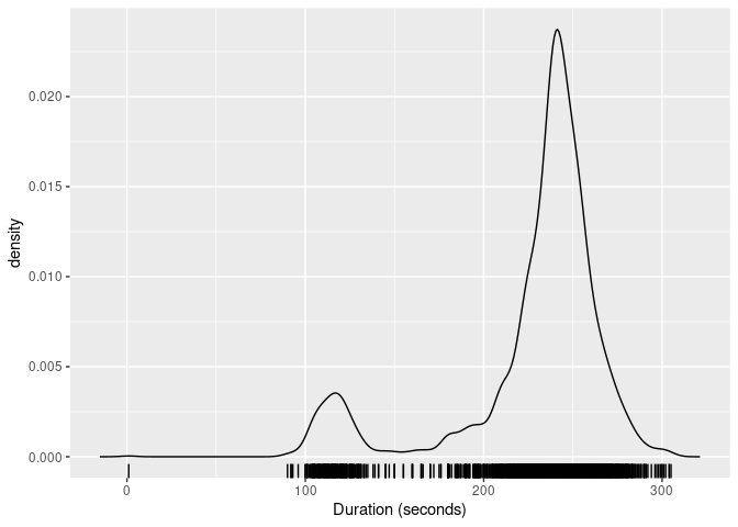
The same functions also work with bivariate data. The figure below
shows the kernel density estimate of the duration and
waiting variables.
oldfaithful |>
  select(duration, waiting) |>
  dist_kde() |>
  gg_density(show_points = TRUE, alpha = 0.15) +
  labs(x = "Duration (seconds)", y = "Waiting time (seconds)")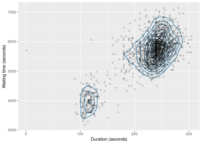
Some old methods of anomaly detection used statistical tests. While these are not recommended, they are still widely used, and are provided in the package for comparison purposes.
oldfaithful |> filter(peirce_anomalies(duration))
#> # A tibble: 2 × 4
#>   time                recorded_duration duration waiting
#>   <dttm>              <chr>                <dbl>   <dbl>
#> 1 2018-04-25 19:08:00 1s                       1    5700
#> 2 2022-12-07 17:19:00 ~4 30s                  30    5220
oldfaithful |> filter(chauvenet_anomalies(duration))
#> # A tibble: 2 × 4
#>   time                recorded_duration duration waiting
#>   <dttm>              <chr>                <dbl>   <dbl>
#> 1 2018-04-25 19:08:00 1s                       1    5700
#> 2 2022-12-07 17:19:00 ~4 30s                  30    5220
oldfaithful |> filter(grubbs_anomalies(duration))
#> # A tibble: 1 × 4
#>   time                recorded_duration duration waiting
#>   <dttm>              <chr>                <dbl>   <dbl>
#> 1 2018-04-25 19:08:00 1s                       1    5700
oldfaithful |> filter(dixon_anomalies(duration))
#> # A tibble: 0 × 4
#> # ℹ 4 variables: time <dttm>, recorded_duration <chr>, duration <dbl>, waiting <dbl>
There are at least three anomalies in this example (due to recording errors), but none of these methods detect them all. An explanation of these tests is provided in Chapter 4 of the book
Boxplots are widely used for anomaly detection. Here are three
variations of boxplots applied to the duration
variable.
oldfaithful |>
  ggplot(aes(x = duration)) +
  geom_boxplot() +
  scale_y_discrete() +
  labs(y = "", x = "Duration (seconds)")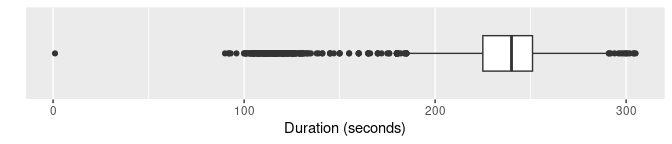
oldfaithful |> gg_hdrboxplot(duration) + labs(x = "Duration (seconds)")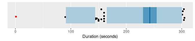
oldfaithful |>
  gg_hdrboxplot(duration, show_points = TRUE) +
  labs(x = "Duration (seconds)")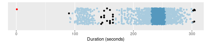
The latter two plots are highest density region (HDR) boxplots, which allow the bimodality of the data to be seen. The dark shaded region contains 50% of the observations, while the lighter shaded region contains 99% of the observations. The plots use vertical jittering to reduce overplotting, and highlight potential outliers (those points lying outside the 99% HDR which have surprisal probability less than 0.0005). An explanation of these plots is provided in Chapter 5 of the book.
It is also possible to produce bivariate boxplots. Several variations are provided in the package. Here are two types of bagplot.
oldfaithful |>
  gg_bagplot(duration, waiting) +
  labs(x = "Duration (seconds)", y = "Waiting time (seconds)")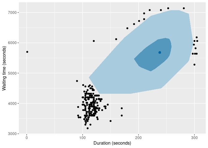
oldfaithful |>
  gg_bagplot(duration, waiting, show_points = TRUE) +
  labs(x = "Duration (seconds)", y = "Waiting time (seconds)")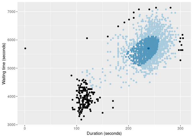
And here are two types of HDR boxplot
oldfaithful |>
  gg_hdrboxplot(duration, waiting) +
  labs(x = "Duration (seconds)", y = "Waiting time (seconds)")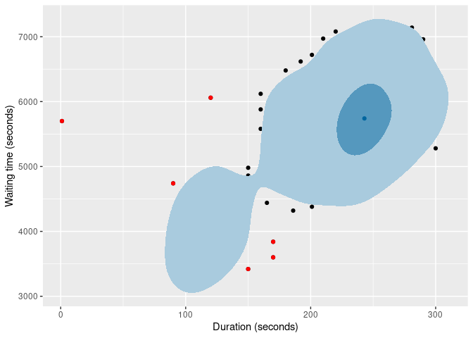
oldfaithful |>
  gg_hdrboxplot(duration, waiting, show_points = TRUE) +
  labs(x = "Duration (seconds)", y = "Waiting time (seconds)")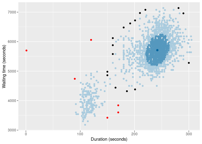
The latter two plots show possible outliers in black (again, defined as points outside the 99% HDR which have surprisal probability less than 0.0005).
Several functions are provided for providing anomaly scores for all observations.
surprisals() function uses either a fitted
statistical model, or a kernel density estimate, to compute
surprisals.surprisals_prob() function computes the probability
of obtaining surprisal values at least as extreme as those
observed.stray_scores() function uses the stray algorithm to
compute anomaly scores.lof_scores() function uses local outlier factors to
compute anomaly scores.glosh_scores() function uses the Global-Local
Outlier Score from Hierarchies algorithm to compute anomaly scores.Here are the top 0.02% most anomalous observations identified by each of the methods.
oldfaithful |>
  mutate(
    surprisal = surprisals(cbind(duration, waiting)),
    surprisal_prob = surprisals_prob(cbind(duration, waiting), approximation = "gpd"),
    strayscore = stray_scores(cbind(duration, waiting)),
    lofscore = lof_scores(cbind(duration, waiting), k = 150),
    gloshscore = glosh_scores(cbind(duration, waiting))
  ) |>
  filter(
    surprisal_prob < 0.002 |
      strayscore > quantile(strayscore, prob = 0.998) |
      lofscore > quantile(lofscore, prob = 0.998) |
      gloshscore > quantile(gloshscore, prob = 0.998)
  ) |>
  arrange(surprisal_prob)
#> # A tibble: 10 × 9
#>    time                recorded_duration    duration waiting surprisal surprisal_prob
#>    <dttm>              <chr>                   <dbl>   <dbl>     <dbl>          <dbl>
#>  1 2022-12-07 17:19:00 ~4 30s                     30    5220      16.4       0.000935
#>  2 2023-07-04 12:03:00 ~1 minute 55ish sec…       60    4920      16.4       0.000967
#>  3 2022-12-03 16:20:00 ~4m                       240    3060      16.4       0.000999
#>  4 2018-04-25 19:08:00 1s                          1    5700      16.4       0.00110
#>  5 2020-09-04 01:38:00 >1m 50s                   110    6240      16.4       0.00112
#>  6 2020-06-01 21:04:00 2 minutes                 120    6060      16.3       0.00145
#>  7 2023-05-26 00:53:00 4m45s                     285    7140      14.9       0.0288
#>  8 2017-09-22 18:51:00 ~281s                     281    7140      14.8       0.0341
#>  9 2023-08-09 20:52:00 4m39s                     279    7140      14.8       0.0345
#> 10 2018-09-22 16:37:00 ~4m13s                    253    7140      14.4       0.0528
#> # ℹ 3 more variables: strayscore <dbl>, lofscore <dbl>, gloshscore <dbl>Some anomaly detection methods require the data to be scaled first,
so all observations are on the same scale. However, many scaling methods
are not robust to anomalies. The mvscale() function
provides a multivariate robust scaling method, that optionally takes
account of the relationships between variables, and uses robust
estimates of center, scale and covariance by default. The centers are
removed using medians, the scale function is the IQR, and the covariance
matrix is estimated using a robust OGK estimate. The data are scaled
using the Cholesky decomposition of the inverse covariance. Then the
scaled data are returned. The scaled variables are rotated to be
orthogonal, so are renamed as z1, z2, etc.
Non-rotated scaling is possible by setting cov = NULL.
mvscale(oldfaithful)
#> Warning in mvscale(oldfaithful): Ignoring non-numeric columns: time,
#> recorded_duration
#> # A tibble: 2,097 × 4
#>    time                recorded_duration      z1     z2
#>    <dttm>              <chr>               <dbl>  <dbl>
#>  1 2017-01-14 00:06:00 3m 16s            -2.20    0.332
#>  2 2017-01-26 14:27:00 ~4m               -0.0431  0.111
#>  3 2017-01-27 23:57:00 2m 1s             -4.27   -3.43
#>  4 2017-01-30 15:09:00 ~4m                0.345  -0.886
#>  5 2017-01-31 13:27:00 ~3.5m             -1.28   -0.332
#>  6 2017-01-31 15:00:00 ~4m                0       0
#>  7 2017-02-03 23:13:00 3m 25s            -1.22   -1.11
#>  8 2017-02-04 22:14:00 3m 34s            -0.966  -0.665
#>  9 2017-02-05 17:19:00 4m 0s             -0.215   0.554
#> 10 2017-02-05 19:00:00 4m 2s             -0.121   0.554
#> # ℹ 2,087 more rows
mvscale(oldfaithful, cov = NULL)
#> Warning in mvscale(oldfaithful, cov = NULL): Ignoring non-numeric columns: time,
#> recorded_duration
#> # A tibble: 2,097 × 4
#>    time                recorded_duration duration waiting
#>    <dttm>              <chr>                <dbl>   <dbl>
#>  1 2017-01-14 00:06:00 3m 16s             -1.98     0.338
#>  2 2017-01-26 14:27:00 ~4m                 0        0.113
#>  3 2017-01-27 23:57:00 2m 1s              -5.37    -3.50
#>  4 2017-01-30 15:09:00 ~4m                 0       -0.902
#>  5 2017-01-31 13:27:00 ~3.5m              -1.35    -0.338
#>  6 2017-01-31 15:00:00 ~4m                 0        0
#>  7 2017-02-03 23:13:00 3m 25s             -1.58    -1.13
#>  8 2017-02-04 22:14:00 3m 34s             -1.17    -0.676
#>  9 2017-02-05 17:19:00 4m 0s               0        0.564
#> 10 2017-02-05 19:00:00 4m 2s               0.0902   0.564
#> # ℹ 2,087 more rows
These binaries (installable software) and packages are in development.
They may not be fully stable and should be used with caution. We make no claims about them.
Health stats visible at Monitor.