The hardware and bandwidth for this mirror is donated by dogado GmbH, the Webhosting and Full Service-Cloud Provider. Check out our Wordpress Tutorial.
If you wish to report a bug, or if you are interested in having us mirror your free-software or open-source project, please feel free to contact us at mirror[@]dogado.de.
2018-04-18
To understand the concept of p value is very important. To teach the the distribution of common statistic( \(\chi^2\) for chisq.test() , t for Student’s t-test , F for F-test) and concept of the p-value, plot.htest() function can be used.
https://cardiomoon.github.io/webr/index.html
You can install this package form the github. Currently, package
webr is under construction and consists of only one
function - plot.htest().
#install.packages("devtools")
devtools::install_github("cardiomoon/webr")The plot.htest() function is a S3 method for class “htest”. Currently, this function covers Welch Two Sample t-test, Pearson’s Chi-squared test, Two Sample t-test, One Sample t-test, Paired t-test and F test to compare two variances.
You can show the distribution of chi-squre statistic and p-value.
 require(moonBook)
 require(webr)

 # chi-squared test
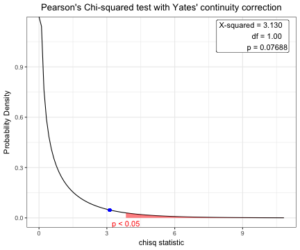
 x=chisq.test(table(acs$sex,acs$DM))
 x
    Pearson's Chi-squared test with Yates' continuity correction

data:  table(acs$sex, acs$DM)
X-squared = 3.1296, df = 1, p-value = 0.07688 plot(x)
You can show the distribution of t-statistic and p-value in one sample t-test.
t.test(acs$age,mu=63)
    One Sample t-test

data:  acs$age
t = 0.77978, df = 856, p-value = 0.4357
alternative hypothesis: true mean is not equal to 63
95 percent confidence interval:
 62.52736 64.09574
sample estimates:
mean of x
63.31155 plot(t.test(acs$age,mu=63))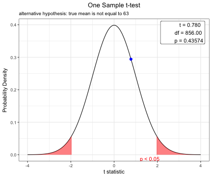
Before performing a t-test, you have to compare two variances.
x=var.test(age~DM,data=acs)
x
    F test to compare two variances

data:  age by DM
F = 1.2383, num df = 552, denom df = 303, p-value = 0.0376
alternative hypothesis: true ratio of variances is not equal to 1
95 percent confidence interval:
 1.012416 1.505776
sample estimates:
ratio of variances
1.238288 plot(x)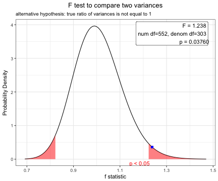
Based on the result of var.test(), you can perform t.test with default option(var.equal=FALSE).
x=t.test(age~DM,data=acs)
x
    Welch Two Sample t-test

data:  age by DM
t = 0.58982, df = 682.36, p-value = 0.5555
alternative hypothesis: true difference in means is not equal to 0
95 percent confidence interval:
 -1.112568  2.068014
sample estimates:
 mean in group No mean in group Yes
63.48101 63.00329 plot(x)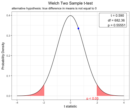
To compare means of body-mass index between male and female patients, perform F test first.
var.test(BMI~sex,data=acs)
    F test to compare two variances

data:  BMI by sex
F = 1.2078, num df = 254, denom df = 508, p-value = 0.07756
alternative hypothesis: true ratio of variances is not equal to 1
95 percent confidence interval:
 0.9794315 1.5008098
sample estimates:
ratio of variances
1.207759 plot(var.test(BMI~sex,data=acs))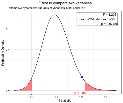 Based on the result of F test, you can perform t-test using pooled
variance.
x=t.test(BMI~sex,data=acs,var.equal=TRUE)
x
    Two Sample t-test

data:  BMI by sex
t = -0.50823, df = 762, p-value = 0.6114
alternative hypothesis: true difference in means is not equal to 0
95 percent confidence interval:
 -0.6348532  0.3737344
sample estimates:
mean in group Female   mean in group Male
24.19492 24.32548 plot(x)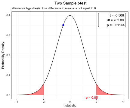
You can show the distribution of t-statistic and p-value in paired t-test.
x=t.test(iris$Sepal.Width,iris$Petal.Width,paired=TRUE)
plot(x)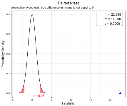
You can change the options of t.test.
x=t.test(BMI~sex, data=acs,conf.level=0.99,alternative="greater",var.equal=TRUE)
plot(x)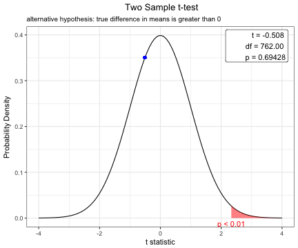
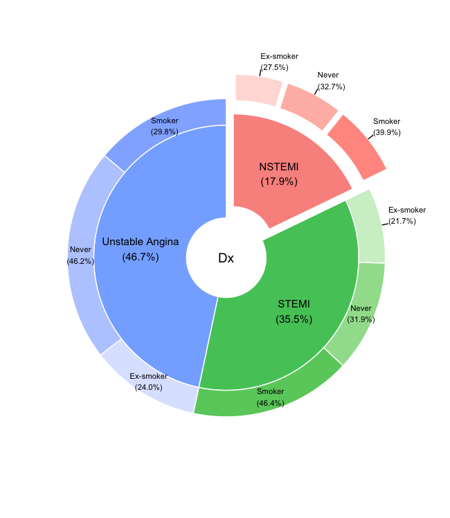
http://rpubs.com/cardiomoon/398623
These binaries (installable software) and packages are in development.
They may not be fully stable and should be used with caution. We make no claims about them.
Health stats visible at Monitor.