The hardware and bandwidth for this mirror is donated by dogado GmbH, the Webhosting and Full Service-Cloud Provider. Check out our Wordpress Tutorial.
If you wish to report a bug, or if you are interested in having us mirror your free-software or open-source project, please feel free to contact us at mirror[@]dogado.de.

valytics

Statistical methods for analytical method comparison and validation studies. The package implements Bland-Altman analysis, Passing-Bablok regression, Deming regression, precision experiments, and quality goal specifications based on biological variation — approaches commonly used in clinical laboratory method validation.

Installation

Install valytics from CRAN:

install.packages("valytics")

Or install the development version from GitHub:

# install.packages("pak")
pak::pak("marcellogr/valytics")

Overview

valytics provides tools for analytical method validation:

Method Comparison - Bland-Altman analysis: Assess agreement through bias and limits of agreement - Passing-Bablok regression: Non-parametric regression robust to outliers - Deming regression: Errors-in-variables regression for method comparison

Precision Experiments - Variance component analysis: Repeatability, intermediate precision, reproducibility - Precision verification: Chi-square test against manufacturer claims - Precision profiles: CV vs concentration modeling with functional sensitivity

Quality Specifications - Biological variation-based goals: Calculate allowable total error from CV_I and CV_G - Sigma metrics: Six Sigma quality assessment - Performance assessment: Evaluate methods against quality specifications

All methods produce publication-ready plots and comprehensive statistical summaries.

Method Comparison Examples

Bland-Altman Analysis

library(valytics)

# Compare two creatinine measurement methods
data(creatinine_serum)

ba <- ba_analysis(
  x = creatinine_serum$enzymatic,
  y = creatinine_serum$jaffe
)

ba
#> 
#> Bland-Altman Analysis
#> ---------------------------------------- 
#> n = 80 paired observations
#> 
#> Difference type: Absolute (y - x)
#> Confidence level: 95%
#> 
#> Results:
#>   Bias (mean difference): 0.174
#>     95% CI: [0.127, 0.220]
#>   SD of differences: 0.209
#> 
#> Limits of Agreement:
#>   Lower LoA: -0.236
#>     95% CI: [-0.316, -0.156]
#>   Upper LoA: 0.584
#>     95% CI: [0.504, 0.663]

plot(ba)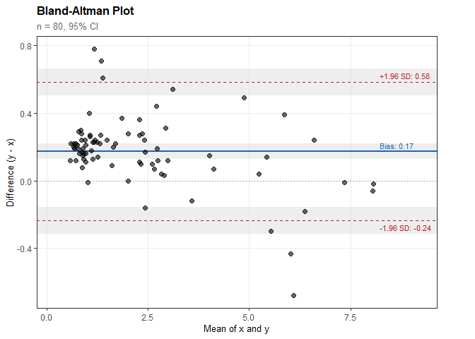

Bland-Altman plot showing differences between Jaffe and enzymatic creatinine methods

Passing-Bablok Regression

pb <- pb_regression(
  x = creatinine_serum$enzymatic,
  y = creatinine_serum$jaffe
)

pb
#> 
#> Passing-Bablok Regression
#> ---------------------------------------- 
#> n = 80 paired observations
#> 
#> CI method: Analytical (Passing-Bablok 1983)
#> Confidence level: 95%
#> 
#> Regression equation:
#>   creatinine_serum$jaffe = 0.234 + 0.971 * creatinine_serum$enzymatic
#> 
#> Results:
#>   Intercept: 0.234
#>     95% CI: [0.229, 0.239]
#>     (excludes 0: significant constant bias)
#> 
#>   Slope: 0.971
#>     95% CI: [0.966, 0.974]
#>     (excludes 1: significant proportional bias)

plot(pb)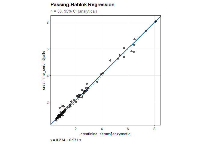

Passing-Bablok regression scatter plot with regression line and confidence band

Deming Regression

dm <- deming_regression(
  x = creatinine_serum$enzymatic,
  y = creatinine_serum$jaffe
)

dm
#> 
#> Deming Regression
#> ---------------------------------------- 
#> n = 80 paired observations
#> 
#> Error ratio (lambda): 1.000
#> CI method: Jackknife
#> Confidence level: 95%
#> 
#> Regression equation:
#>   creatinine_serum$jaffe = 0.277 + 0.953 * creatinine_serum$enzymatic
#> 
#> Results:
#>   Intercept: 0.277 (SE = 0.028)
#>     95% CI: [0.222, 0.332]
#>     (excludes 0: significant constant bias)
#> 
#>   Slope: 0.953 (SE = 0.014)
#>     95% CI: [0.925, 0.982]
#>     (excludes 1: significant proportional bias)

plot(dm)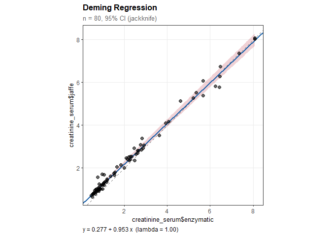

Deming regression scatter plot with regression line and confidence band

Precision Experiments

Variance Component Analysis

# Analyze precision from a multi-day, multi-run study
data(troponin_precision)

prec <- precision_study(
  data = troponin_precision,
  value = "value",
  sample = "level",
  day = "day",
  run = "run"
)

prec
#> 
#> Precision Study Analysis
#> --------------------------------------------- 
#> n = 120 observations
#> Design: day/run/replicate (inferred)
#> Estimation: ANOVA (Method of Moments)
#> CI method: Satterthwaite, 95% CI
#> 
#> Samples: 6 concentration levels
#> (Showing results for first sample; use $by_sample for all)
#> 
#> Precision Estimates:
#> --------------------------------------------- 
#>   Repeatability:       SD = 0.243  (CV = 4.86%)
#>                        95% CI: [0.170, 0.426]
#>   Between-run:         SD = 0.188  (CV = 3.76%)
#>                        95% CI: [0.117, 0.461]
#>   Between-day:         SD = 0.000  (CV = 0.00%)
#>                        95% CI: [0.000, 0.000]
#>   Within-laboratory precision: SD = 0.307  (CV = 6.15%)
#>                        95% CI: [0.227, 0.476]

plot(prec, type = "cv")
#> Warning in data.frame(sample = sample_names[i], mean_conc = if
#> (!is.null(sample_means)) sample_means[sample_names[i]] else i, : Zeilennamen
#> wurden in einer short Variablen gefunden und wurden verworfen

#> Warning in data.frame(sample = sample_names[i], mean_conc = if
#> (!is.null(sample_means)) sample_means[sample_names[i]] else i, : Zeilennamen
#> wurden in einer short Variablen gefunden und wurden verworfen

#> Warning in data.frame(sample = sample_names[i], mean_conc = if
#> (!is.null(sample_means)) sample_means[sample_names[i]] else i, : Zeilennamen
#> wurden in einer short Variablen gefunden und wurden verworfen

#> Warning in data.frame(sample = sample_names[i], mean_conc = if
#> (!is.null(sample_means)) sample_means[sample_names[i]] else i, : Zeilennamen
#> wurden in einer short Variablen gefunden und wurden verworfen

#> Warning in data.frame(sample = sample_names[i], mean_conc = if
#> (!is.null(sample_means)) sample_means[sample_names[i]] else i, : Zeilennamen
#> wurden in einer short Variablen gefunden und wurden verworfen

#> Warning in data.frame(sample = sample_names[i], mean_conc = if
#> (!is.null(sample_means)) sample_means[sample_names[i]] else i, : Zeilennamen
#> wurden in einer short Variablen gefunden und wurden verworfen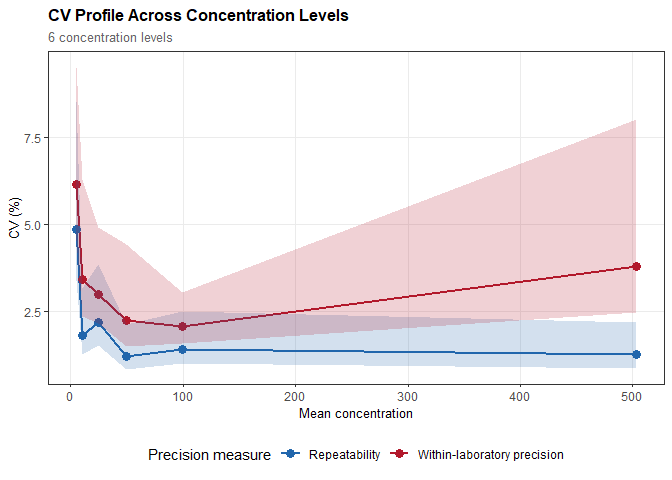

CV profile showing precision measures with confidence intervals

Precision Profiles and Functional Sensitivity

# Model CV vs concentration relationship
prof <- precision_profile(prec, cv_target = 10)

prof
#> 
#> Precision Profile Analysis
#> ---------------------------------------- 
#> n = 6 concentration levels
#> Concentration range: 5 to 503 (100.75-fold)
#> 
#> Model: Hyperbolic
#>   CV = sqrt(2.667^2 + (26.905/x)^2)
#> 
#> Parameters:
#>   a = 2.667
#>   b = 26.905
#> 
#> Fit Quality:
#>   R-squared = 0.816
#>   RMSE = 0.578
#> 
#> Functional Sensitivity:
#>   CV = 10%: concentration = 2.792

plot(prof)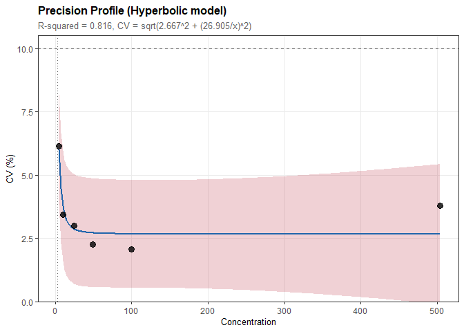

Quality Specifications

Allowable Total Error from Biological Variation

Calculate performance goals based on within-subject (CV_I) and between-subject (CV_G) biological variation:

# Creatinine biological variation (from EFLM database)
# CV_I = 5.95%, CV_G = 14.7%
ate <- ate_from_bv(cvi = 5.95, cvg = 14.7)

ate
#> 
#> Analytical Performance Specifications from Biological Variation
#> ------------------------------------------------------------ 
#> 
#> Input:
#>   Within-subject CV (CV_I): 5.95%
#>   Between-subject CV (CV_G): 14.70%
#>   Performance level: desirable
#>   Coverage factor (k): 1.65
#> 
#> Specifications:
#>   Allowable imprecision (CV_A): 2.98%
#>   Allowable bias: 3.96%
#>   Total allowable error (TEa): 8.87%

Six Sigma Quality Assessment

# Evaluate method performance
sm <- sigma_metric(bias = 1.5, cv = 2.5, tea = 10)

sm
#> 
#> Six Sigma Metric
#> ---------------------------------------- 
#> 
#> Input:
#>   Observed bias: 1.50%
#>   Observed CV: 2.50%
#>   Total allowable error (TEa): 10.00%
#> 
#> Result:
#>   Sigma: 3.40
#>   Performance: Marginal
#>   Defect rate: ~66,800 per million

Performance Assessment

# Full quality assessment
assess <- ate_assessment(
  bias = 1.5, 
  cv = 2.5, 
  tea = 10,
  allowable_bias = 4.0, 
  allowable_cv = 3.0
)

assess
#> 
#> Analytical Performance Assessment
#> -------------------------------------------------- 
#> 
#>   >>> METHOD ACCEPTABLE <<<
#> 
#> Performance Summary:
#>   Parameter              Observed  Allowable     Status
#>   -------------------- ---------- ---------- ----------
#>   Bias                      1.50%      4.00%       PASS
#>   CV (Imprecision)          2.50%      3.00%       PASS
#>   Total Error               5.62%     10.00%       PASS
#> 
#> Sigma Metric: 3.40 (Marginal)

Features

Multiple interfaces: Vector input or formula syntax (method1 ~ method2)
Flexible CI methods: Analytical, Satterthwaite, or bootstrap BCa confidence intervals
Assumption checking: CUSUM linearity test, Shapiro-Wilk normality test
Precision analysis: ANOVA and REML variance component estimation
Quality goals: Biological variation-based specifications (optimal/desirable/minimum)
Publication-ready plots: Built on ggplot2, fully customizable
Tidy workflows: Consistent API, informative summaries

Example Datasets

The package includes four realistic clinical datasets:

Dataset	Description	n
`glucose_methods`	POC meter vs. laboratory analyzer	60
`creatinine_serum`	Enzymatic vs. Jaffe methods	80
`troponin_cardiac`	Two hs-cTnI platforms	50
`troponin_precision`	hs-cTnI precision study (6 levels)	120

Vignettes

Method Comparison Workflow: Step-by-step analysis guide
Understanding Method Comparison Statistics: Educational overview
Deming Regression: When and how to use errors-in-variables regression
Quality Goals from Biological Variation: Setting performance specifications
Precision Profiles and Functional Sensitivity: CV modeling and functional sensitivity

References

Bland-Altman:

Bland JM, Altman DG (1986). Statistical methods for assessing agreement between two methods of clinical measurement. Lancet, 1(8476):307-310.
Bland JM, Altman DG (1999). Measuring agreement in method comparison studies. Statistical Methods in Medical Research, 8(2):135-160.

Passing-Bablok:

Passing H, Bablok W (1983). A new biometrical procedure for testing the equality of measurements from two different analytical methods. Journal of Clinical Chemistry and Clinical Biochemistry, 21(11):709-720.

Deming:

Linnet K (1990). Estimation of the linear relationship between the measurements of two methods with proportional errors. Statistics in Medicine, 9(12):1463-1473.

Precision:

Chesher D (2008). Evaluating assay precision. Clinical Biochemistry Reviews, 29(Suppl 1):S23-S26.
Kroll MH, Emancipator K (1993). A theoretical evaluation of linearity. Clinical Chemistry, 39(3):405-413.

Biological Variation:

Fraser CG, Petersen PH (1993). Desirable standards for laboratory tests if they are to fulfill medical needs. Clinical Chemistry, 39(7):1447-1453.
EFLM Biological Variation Database: https://biologicalvariation.eu/

License

GPL-3

These binaries (installable software) and packages are in development.
They may not be fully stable and should be used with caution. We make no claims about them.
Health stats visible at Monitor.