The hardware and bandwidth for this mirror is donated by dogado GmbH, the Webhosting and Full Service-Cloud Provider. Check out our Wordpress Tutorial.
If you wish to report a bug, or if you are interested in having us mirror your free-software or open-source project, please feel free to contact us at mirror[@]dogado.de.
twfeivdecomp is a package for decomposing the two-way
fixed effects instrumental variable (TWFEIV) estimator under staggered
instrumented difference-in-differences (DID-IV) designs.
The package decomposes the TWFEIV estimator into a weighted average of
all possible Wald-DID estimators, providing a transparent view of how
different 2x2 comparisons contribute to the overall estimate.
The decomposition can be performed both with and without time-varying controls.
You can install the development version of twfeivdecomp from GitHub:
library(devtools)
install_github("shomiyaji/twfeiv-decomp")-twfeiv_decomp(): decomposes the TWFEIV estimator into
all possible Wald-DID estimators, with or without time-varying
controls.
The package includes an example dataset simulation_data,
which is a small simulated panel dataset.
It contains 72 observations (12 units observed over 6 time periods) with
the following variables:
id: Unit identifiertime: Time period (2000–2005)instrument: Binary instrument variabletreatment: Treatment variableoutcome: Outcome variablecontrol1, control2: Additional control
variablesThis is a basic example which shows how to decompose the TWFEIV
estimator into its Wald-DID components using the
twfeivdecomp package.
library(twfeivdecomp)
decomposition_result <- twfeiv_decomp(outcome ~ treatment | instrument,
data = simulation_data,
id_var = "id",
time_var = "time",
summary_output = F)
# Decomposition result
head(decomposition_result)
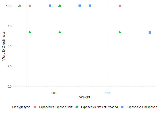
#> exposed_cohort unexposed_cohort design_type Wald_DID_estimate
#> 1 2001 2002 Exposed vs Not Yet Exposed 6.666667
#> 2 2005 2002 Exposed vs Exposed Shift 10.000000
#> 3 2003 2002 Exposed vs Exposed Shift 10.000000
#> 4 2002 2001 Exposed vs Exposed Shift 10.000000
#> 5 2005 2001 Exposed vs Exposed Shift 10.000000
#> 6 2003 2001 Exposed vs Exposed Shift 10.000000
#> weight
#> 1 0.02777778
#> 2 0.02777778
#> 3 0.02777778
#> 4 0.07407407
#> 5 0.07407407
#> 6 0.11111111
# Print the summary
print_summary(data = decomposition_result, return_df = FALSE)
#> # A tibble: 3 × 3
#> design_type weight_sum Weighted_average_Wald_DID
#> <chr> <dbl> <dbl>
#> 1 Exposed vs Exposed Shift 0.333 10
#> 2 Exposed vs Not Yet Exposed 0.324 8
#> 3 Exposed vs Unexposed 0.343 8.65
# Print the figure
library(ggplot2)
ggplot(decomposition_result) +
aes(x = weight, y = Wald_DID_estimate,
shape = factor(design_type),
color = factor(design_type)) +
geom_point(size = 3) +
geom_hline(yintercept = 0, linetype = "dashed") +
theme_minimal() +
labs(x = "Weight", y = "Wald DID estimate",
shape = "Design type", color = "Design type") +
theme(
legend.position = "bottom",
legend.box = "horizontal"
)
Miyaji, Sho. (2024). Instrumented Difference-in-Differences
with Heterogeneous Treatment Effects.
arXiv:2405.12083. Available at: https://arxiv.org/abs/2405.12083
Miyaji, Sho. (2024). Two-Way Fixed Effects Instrumental
Variable Regressions in Staggered DID-IV Designs.
arXiv:2405.16467. Available at: https://arxiv.org/abs/2405.16467
These binaries (installable software) and packages are in development.
They may not be fully stable and should be used with caution. We make no claims about them.
Health stats visible at Monitor.