The hardware and bandwidth for this mirror is donated by dogado GmbH, the Webhosting and Full Service-Cloud Provider. Check out our Wordpress Tutorial.
If you wish to report a bug, or if you are interested in having us mirror your free-software or open-source project, please feel free to contact us at mirror[@]dogado.de.
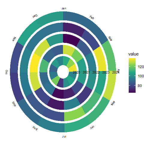
The goal of tsspiral is to create spiral version of time series plots.
You can install the development version of tsspiral from GitHub with:
# install.packages("pak")
pak::pak("thiyangt/tsspiralplot")library(tsspiral)
library(ggplot2)
library(viridis)
#> Loading required package: viridisLite
monthly_data <- data.frame(
date = seq.Date(
as.Date("2020-01-01"),
as.Date("2024-12-01"),
by = "month"
)
)
monthly_data$value <- rnorm(
nrow(monthly_data),
mean = 100,
sd = 20
)
ggplot(
monthly_data,
aes(
x = date,
y = value,
fill = value
)
) +
geom_tsspiral(
ring_spacing = 2
) +
scale_fill_viridis_c() +
theme_void()
ggplot(
  monthly_data,
  aes(
    x = date,
    y = value,
    fill = value
  )
) +
  geom_tsspiral(
    ring_spacing = 1
  ) +
  scale_fill_viridis_c() +
  theme_void()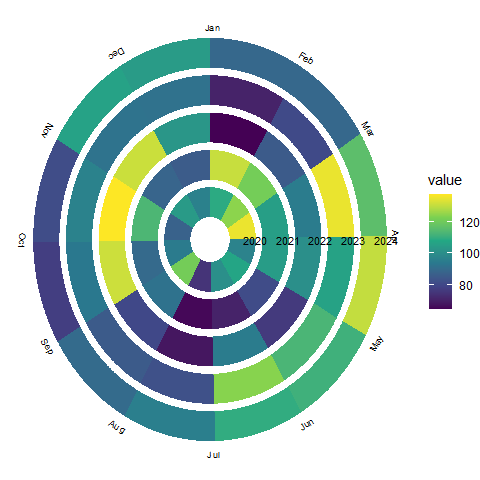
monthly_data <- data.frame(
  date = seq.Date(
    as.Date("2020-02-01"),
    as.Date("2024-12-01"),
    by = "month"
  )
)

monthly_data$value <- rnorm(
  nrow(monthly_data),
  mean = 100,
  sd = 20
)

ggplot(
  monthly_data,
  aes(
    x = date,
    y = value,
    fill = value
  )
) +
  geom_tsspiral(
    ring_spacing = 2
  ) +
  scale_fill_viridis_c() +
  theme_void()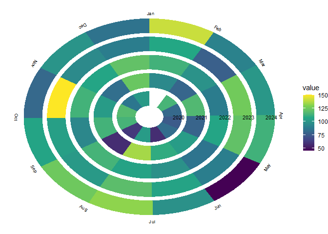
quarterly_data <- data.frame(
  date = seq.Date(
    as.Date("2020-01-01"),
    as.Date("2025-10-01"),
    by = "quarter"
  )
)

quarterly_data$value <- rnorm(
  nrow(quarterly_data),
  100,
  20
)

ggplot(
  quarterly_data,
  aes(
    x = date,
    y = value,
    fill = value
  )
) +
  geom_tsspiral(
    ring_spacing = 2
  ) +
  scale_fill_viridis_c() +
  theme_void()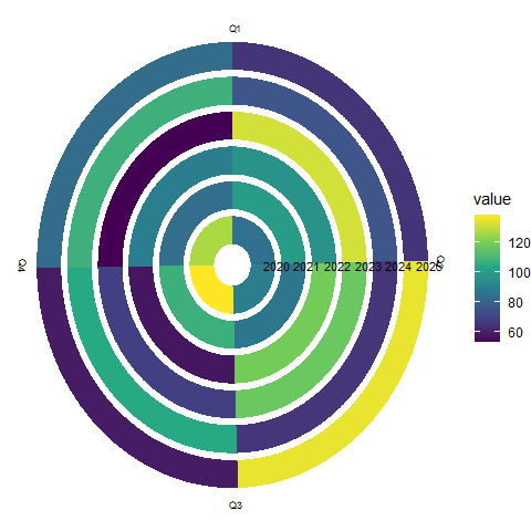
weekly_data <- data.frame(
  date = seq.Date(
    as.Date("2023-01-01"),
    as.Date("2025-12-28"),
    by = "week"
  )
)

weekly_data$value <- rnorm(
  nrow(weekly_data),
  100,
  20
)

ggplot(
  weekly_data,
  aes(
    x = date,
    y = value,
    fill = value
  )
) +
  geom_tsspiral(
    ring_spacing = 2
  ) +
  scale_fill_viridis_c() +
  theme_void()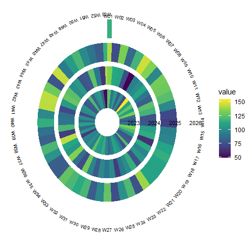
set.seed(123)

dat <- data.frame(
  date = seq.Date(
   as.Date("2020-01-01"),
   as.Date("2023-12-31"),
    by = "day"
   )
 )

dat$value <- 100 +
 20 * sin(
    2 * pi *
       lubridate::yday(dat$date) / 365
   ) +
  rnorm(
     nrow(dat),
     sd = 5
   )

 ggplot(
  dat,
  aes(
    x = date,
    y = value,
   fill = value
  ) ) +
  geom_tsspiral(
    ring_spacing = 2
   ) +
   scale_fill_viridis_c() +
   theme_void()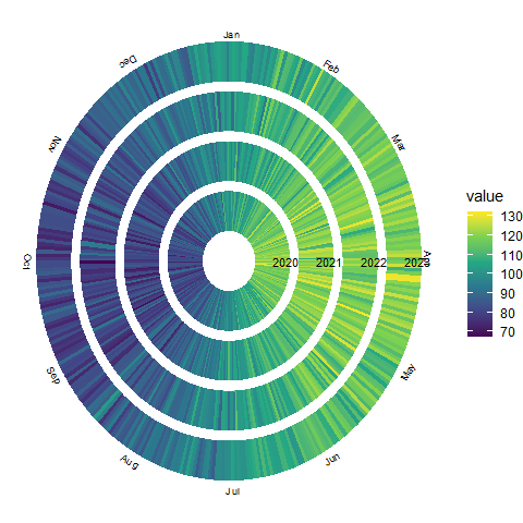
set.seed(123)

dat <- data.frame(
  date = seq.Date(
    as.Date("2020-01-01"),
    as.Date("2023-12-31"),
    by = "day"
  )
)

doy <- lubridate::yday(dat$date)

dat$value <-
  20 +
  15 * sin(2 * pi * doy / 365) +
  35 * exp(-((doy - 100) / 20)^2) +
  25 * exp(-((doy - 280) / 30)^2) +
  rnorm(nrow(dat), 0, 3)

ggplot(
  dat,
  aes(
    x = date,
    y = value,
    fill = value
  )
) +
  geom_tsspiralbar(
    ring_spacing = 2
  ) +
  scale_fill_viridis_c() +
  theme_void()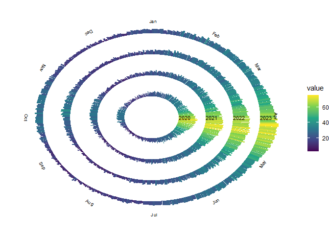
library(ggplot2)

set.seed(123)

dat <- data.frame(
  date = seq.Date(
    as.Date("2020-01-01"),
    as.Date("2023-12-31"),
    by = "day"
  )
)

dat$value <- 100 +
  30 * sin(
    2 * pi * lubridate::yday(dat$date) / 365
  ) +
  rnorm(
    nrow(dat),
    sd = 8
  )

ggplot(
  dat,
  aes(
    x = date,
    y = value,
    fill = value
  )
) +
  geom_tsspiralbar(
    ring_spacing = 2
  ) +
  scale_fill_viridis_c() +
  theme_void()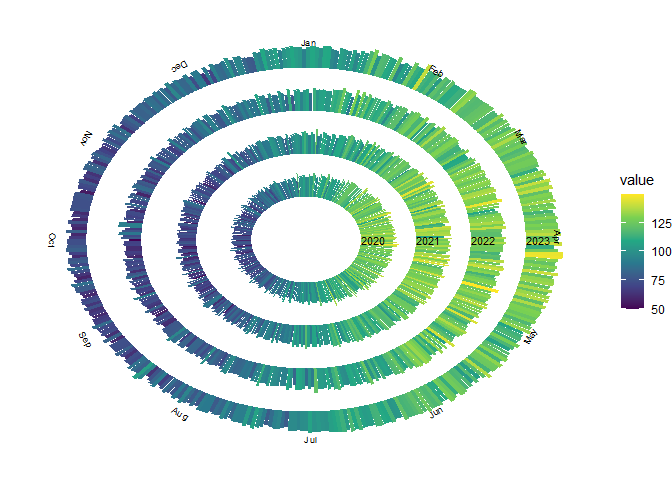
library(ggplot2)

set.seed(123)

# Generate a daily time series
spiral_dat <- data.frame(
  date = seq.Date(
    from = as.Date("2020-01-01"),
    to = as.Date("2023-12-31"),
    by = "day"
  )
)

# Generate a seasonal time series
spiral_dat$value <-
  100 +
  25 * sin(
    2 * pi * lubridate::yday(spiral_dat$date) / 365
  ) +
  rnorm(
    nrow(spiral_dat),
    sd = 5
  )

# Create missing periods
missing_dates <- c(
  seq.Date(
    as.Date("2020-03-01"),
    as.Date("2020-03-20"),
    by = "day"
  ),
  seq.Date(
    as.Date("2021-07-10"),
    as.Date("2021-08-05"),
    by = "day"
  ),
  seq.Date(
    as.Date("2023-01-15"),
    as.Date("2023-02-10"),
    by = "day"
  )
)

# Remove missing observations
spiral_dat <- spiral_dat[
  !spiral_dat$date %in% missing_dates,
]

# Plot missingness
ggplot(
  spiral_dat,
  aes(x = date)
) +
  geom_tsspiralmiss(
    ring_spacing = 2,
    observed_colour = "grey85",
    missing_colour = "black"
  ) +
  theme_void()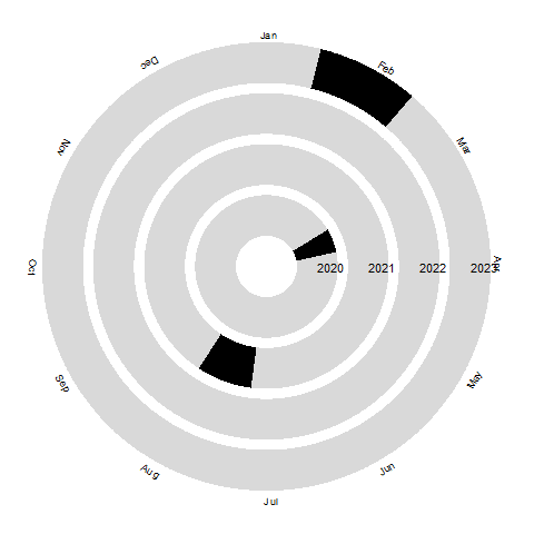
# =========================================================
# Example: Two months of hourly data
# =========================================================

set.seed(123)

hourly_data <- tibble::tibble(
  datetime = seq(
    from = as.POSIXct("2026-01-01 00:00"),
    to   = as.POSIXct("2026-02-28 23:00"),
    by   = "hour"
  )
) |>
  dplyr::mutate(
    hour = lubridate::hour(datetime),
    day = lubridate::day(datetime),

    temperature =
      25 +
      4 * sin(2 * pi * hour / 24) +
      0.05 * day +
      stats::rnorm(
        length(datetime),
        0,
        0.8
      )
  )
# January
calendar_hourly_polar(
  hourly_data,
  datetime,
  temperature,
  month = "2026-01-01"
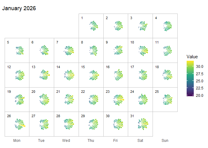
)
# February
calendar_hourly_polar(
  hourly_data,
  datetime,
  temperature,
  month = "2026-02-01"
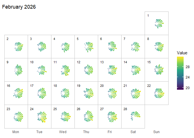
)
set.seed(123)

dat <- data.frame(
  date = seq.Date(
    from = as.Date("2020-01-01"),
    to = as.Date("2023-12-31"),
    by = "day" ))

dat$value <- 20 +
  5 * sin(
    2 * pi * lubridate::yday(dat$date) / 365.25
  ) +
   rnorm(nrow(dat), 0, 1)

temporal_hierarchical(
 data = dat,
 date = date,
 value = value)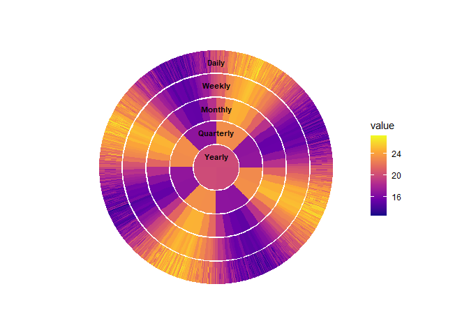
These binaries (installable software) and packages are in development.
They may not be fully stable and should be used with caution. We make no claims about them.
Health stats visible at Monitor.