The hardware and bandwidth for this mirror is donated by dogado GmbH, the Webhosting and Full Service-Cloud Provider. Check out our Wordpress Tutorial.
If you wish to report a bug, or if you are interested in having us mirror your free-software or open-source project, please feel free to contact us at mirror[@]dogado.de.
![]()
![]()
![]()
triplediff is an R package for computing average treatment effects in Triple Differences Designs (also known as Difference-in-Differences-in-Differences or DDD). DDD designs are widely used in empirical work to relax parallel trends assumptions in Difference-in-Differences settings. This package provides functions to estimate group-time average treatment effect and event-study type estimands associated with DDD designs. The setups allowed are:
The triplediff package implements the framework proposed
in:
You can install the latest development version of
triplediff from Github with:
# install.packages("devtools")
devtools::install_github("marcelortizv/triplediff")

library(triplediff)triplediffWe provide a quick start example to illustrate the main features of
the package. The UX is designed to be similar to the did
package, so users familiar with it should feel comfortable using
triplediff.
ddd is the main function for computing the DDD
estimators proposed in Ortiz-Villavicencio and
Sant’Anna (2025). At its core, ddd employs regression
adjustment, inverse probability weighing, and doubly robust estimators
that are valid under conditional DDD parallel trends.
To use ddd, the minimal data requirements include:
id: Unit unique identifier (e.g., firm, individual,
etc.). Its column name is associated with parameter
idname.
period: Time identifier (e.g., year, month, etc.).
Its column name is associated with parameter
tname.
outcome: Outcome variable of interest. Its column
name is associated with parameter yname.
state: First period when treatment is enabled for a
particular unit. It is a positive number for treated units and defines
which group the unit belongs to. It takes value 0 or
Inf for never-enabling units. Its column name is associated
with parameter gname.
partition: This is an indicator variable that is 1
for the units eligible for treatment and 0 otherwise. Its column name is
associated with parameter pname.
The following are two simplified examples of how to use the
ddd function. The first one is for a two-period DDD setup,
while the second one is for a multiple-period DDD setup with staggered
treatment adoption.
First, we simulate some data with a built-in function
gen_dgp_2periods that generates a two-period DDD setup with
a single treatment date. This function receives the number of units and
the type of DGP design to generate. The gen_dgp_2periods
function returns a data frame with the required columns for the
ddd function with 4 covariates.
set.seed(1234) # Set seed for reproducibility
# Simulate data for a two-periods DDD setup
df <- gen_dgp_2periods(
  size = 5000, # Number of units
  dgp_type = 1 # Type of DGP design
)$data

head(df)
#> Key: <id>
#>       id state partition  time        y        cov1       cov2      cov3
#>    <int> <num>     <num> <int>    <num>       <num>      <num>     <num>
#> 1:     1     0         0     1 209.9152 -0.97080934 -1.1726958 2.3893945
#> 2:     1     0         0     2 417.5260 -0.97080934 -1.1726958 2.3893945
#> 3:     2     0         0     1 211.4919  0.02591115  0.2763066 0.1063123
#> 4:     2     0         0     2 420.3656  0.02591115  0.2763066 0.1063123
#> 5:     3     0         0     1 221.9431  0.97147321 -0.4292088 0.5012794
#> 6:     3     0         0     2 440.9623  0.97147321 -0.4292088 0.5012794
#>          cov4 cluster
#>         <num>   <int>
#> 1:  0.2174955      39
#> 2:  0.2174955      39
#> 3: -0.1922253      29
#> 4: -0.1922253      29
#> 5:  1.1027248      44
#> 6:  1.1027248      44
Now we can estimate the average treatment effect on the treated (ATT)
using the ddd function.
# Estimate the average treatment effect on the treated, ATT(2,2)

att_22 <- ddd(yname = "y", tname = "time", idname = "id", gname = "state",
             pname = "partition", xformla = ~cov1 + cov2 + cov3 + cov4,
             data = df, control_group = "nevertreated", est_method = "dr")

summary(att_22)
#>  Call:
#> ddd(yname = "y", tname = "time", idname = "id", gname = "state",
#>     pname = "partition", xformla = ~cov1 + cov2 + cov3 + cov4,
#>     data = df, control_group = "nevertreated", est_method = "dr")
#> =========================== DDD Summary ==============================
#>  DR-DDD estimation for the ATT:
#>      ATT       Std. Error    Pr(>|t|)  [95% Ptwise. Conf. Band]
#>     -0.0780       0.0828       0.3463      -0.2404       0.0843
#>
#>  Note: * indicates that the confidence interval does not contain zero.
#>  --------------------------- Data Info   -----------------------------
#>  Panel Data
#>  Outcome variable: y
#>  Qualification variable: partition
#>  No. of units at each subgroup:
#>    treated-and-eligible: 1232
#>    treated-but-ineligible: 1285
#>    eligible-but-untreated: 1256
#>    untreated-and-ineligible: 1227
#>  --------------------------- Algorithms ------------------------------
#>  Outcome Regression estimated using: OLS
#>  Propensity score estimated using: Maximum Likelihood
#>  --------------------------- Std. Errors  ----------------------------
#>  Level of significance:  0.05
#>  Analytical standard errors.
#>  Type of confidence band:  Pointwise Confidence Interval
#>  =====================================================================
#> See Ortiz-Villavicencio and Sant'Anna (2025) for details.Next, we can simulate some data with a built-in function
gen_dgp_mult_periods that generates a multiple-period DDD
setup with staggered treatment adoption. This function receives the
number of units and the type of DGP design to generate. The
gen_dgp_mult_periods function returns a data frame with the
required columns for the ddd function with 4
covariates.
set.seed(1234) # Set seed for reproducibility
# Simulate data for a multiple-period DDD setup with staggered treatment adoption
data <- gen_dgp_mult_periods(size = 500, dgp_type = 1)$data

head(data)
#> Key: <id>
#>       id state partition  time         y        cov1       cov2       cov3
#>    <int> <num>     <num> <int>     <num>       <num>      <num>      <num>
#> 1:     1     3         1     1 1371.1923 -0.97080934  1.3995704 1.48834130
#> 2:     1     3         1     2 1690.9157 -0.97080934  1.3995704 1.48834130
#> 3:     1     3         1     3 2034.5661 -0.97080934  1.3995704 1.48834130
#> 4:     2     2         1     1  934.0812  0.02591115 -0.9747527 0.01714001
#> 5:     2     2         1     2 1189.5495  0.02591115 -0.9747527 0.01714001
#> 6:     2     2         1     3 1444.1072  0.02591115 -0.9747527 0.01714001
#>          cov4 cluster
#>         <num>   <int>
#> 1:  0.3853346      27
#> 2:  0.3853346      27
#> 3:  0.3853346      27
#> 4: -0.7822000      45
#> 5: -0.7822000      45
#> 6: -0.7822000      45
Now we can estimate the group-time average treatment effect on the
treated using the ddd function.
# Estimate the group-time average treatment effect in DDD

att_gt <- ddd(yname = "y", tname = "time", idname = "id", gname = "state",
              pname = "partition", xformla = ~cov1 + cov2 + cov3 + cov4,
              data = data, control_group = "nevertreated",
              base_period = "universal", est_method = "dr")

summary(att_gt)
#>  Call:
#> ddd(yname = "y", tname = "time", idname = "id", gname = "state",
#>     pname = "partition", xformla = ~cov1 + cov2 + cov3 + cov4,
#>     data = data, control_group = "nevertreated", base_period = "universal",
#>     est_method = "dr")
#> =========================== DDD Summary ==============================
#>  DR-DDD estimation for the ATT(g,t):
#> Group Time  ATT(g,t)  Std. Error [95% Pointwise  Conf. Band]
#>   2    1       0.0000         NA           NA            NA
#>   2    2      10.4901     0.3613       9.7819       11.1983  *
#>   2    3      20.5986     0.3868      19.8405       21.3568  *
#>   3    1      -0.4593     0.3660      -1.1767        0.2580
#>   3    2       0.0000         NA           NA            NA
#>   3    3      24.5983     0.3333      23.9450       25.2515  *
#>
#>  Note: * indicates that the confidence interval does not contain zero.
#>  --------------------------- Data Info   -----------------------------
#>  Panel Data
#>  Outcome variable: y
#>  Qualification variable: partition
#>  Control group: Never Treated
#>  No. of units per treatment group:
#>   Units enabling treatment at period 3: 198
#>   Units enabling treatment at period 2: 195
#>   Units never enabling treatment: 107
#>  --------------------------- Algorithms ------------------------------
#>  Outcome Regression estimated using: OLS
#>  Propensity score estimated using: Maximum Likelihood
#>  --------------------------- Std. Errors  ----------------------------
#>  Level of significance:  0.05
#>  Analytical standard errors.
#>  Type of confidence band:  Pointwise Confidence Interval
#>  =====================================================================
#>  See Ortiz-Villavicencio and Sant'Anna (2025) for details.
Then, we can aggregate the group-time average treatment effect on the
treated to obtain the event-study type estimates. The
agg_ddd function allows us to aggregate the results from
the ddd function.
es_e <- agg_ddd(att_gt, type = "eventstudy")

summary(es_e)
#>  Call:
#> agg_ddd(ddd_obj = att_gt, type = "eventstudy")
#> ========================= DDD Aggregation ============================
#>  Overall summary of ATT's based on event-study/dynamic aggregation:
#>      ATT    Std. Error     [ 95%  Conf. Int.]
#>  19.0983        0.3213    18.4685     19.7281 *
#>
#>  Event Study:
#>  Event time Estimate Std. Error [95% Ptwise.  Conf. Band]
#>          -2  -0.4593     0.3660       -1.1767      0.2580
#>          -1   0.0000         NA            NA          NA
#>           0  17.5980     0.4095       16.7955     18.4005 *
#>           1  20.5986     0.3868       19.8405     21.3568 *
#>
#>  Note: * indicates that the confidence interval does not contain zero.
#>  --------------------------- Data Info   -----------------------------
#>  Outcome variable: y
#>  Qualification variable: partition
#>  Control group:  Never Treated
#>  --------------------------- Std. Errors  ----------------------------
#>  Level of significance:  0.05
#>  Analytical standard errors.
#>  =====================================================================
#>  See Ortiz-Villavicencio and Sant'Anna (2025) for details.
From these event-study type estimates, we can plot the results using
the ggplot library to create crisp visualizations.
es_df <- with(es_e$aggte_ddd, {
    tibble::tibble(period   = egt,
                   estimate = att.egt,
                   ci_lower = estimate - crit.val.egt * se.egt,
                   ci_upper = estimate + crit.val.egt * se.egt)
  })


all_per <- sort(unique(es_df$period))

p <- ggplot(es_df, aes(period, estimate)) +
    geom_errorbar(aes(ymin = ci_lower, ymax = ci_upper),
                  width = .15,
                  position = position_dodge(width = .3)) +
    geom_point(size = 2.2,
               position = position_dodge(width = .3)) +
    geom_hline(yintercept = 0, linewidth = .3) +
    geom_vline(xintercept = -1, linetype = "dashed",
               linewidth = .3) +
    scale_x_continuous(
      breaks = all_per
    ) +
         labs(title = "",
         x = "Event Time",
         y = "Treatment Effect") +
    theme_bw(base_size = 12) +
    theme(plot.title   = element_text(hjust = .25),
          legend.position = "right")

  p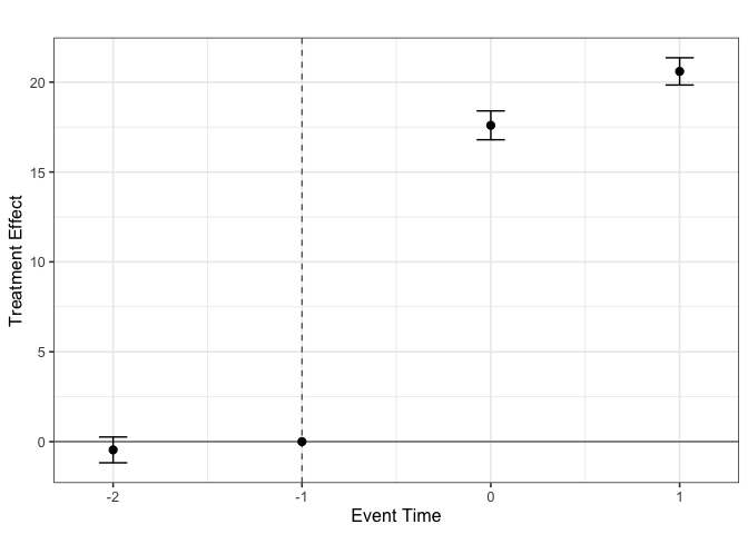
Finally, we can also estimate the group-time average treatment effect
using a GMM-based estimator with not-yet-treated units as comparison
group. This is done by setting the control_group parameter
to "notyettreated" in the ddd function.
# do the same but using GMM-based notyettreated
att_gt_nyt <- ddd(yname = "y", tname = "time", idname = "id", gname = "state",
              pname = "partition", xformla = ~cov1 + cov2 + cov3 + cov4,
              data = data, control_group = "notyettreated",
              base_period = "universal", est_method = "dr")

summary(att_gt_nyt)
#>  Call:
#> ddd(yname = "y", tname = "time", idname = "id", gname = "state",
#>     pname = "partition", xformla = ~cov1 + cov2 + cov3 + cov4,
#>     data = data, control_group = "notyettreated", base_period = "universal",
#>     est_method = "dr")
#> =========================== DDD Summary ==============================
#>  DR-DDD estimation for the ATT(g,t):
#> Group Time  ATT(g,t)  Std. Error [95% Pointwise  Conf. Band]
#>   2    1       0.0000         NA           NA            NA
#>   2    2      10.1894     0.2759       9.6486       10.7302  *
#>   2    3      20.5986     0.3868      19.8405       21.3568  *
#>   3    1      -0.4593     0.3660      -1.1767        0.2580
#>   3    2       0.0000         NA           NA            NA
#>   3    3      24.5983     0.3333      23.9450       25.2515  *
#>
#>  Note: * indicates that the confidence interval does not contain zero.
#>  --------------------------- Data Info   -----------------------------
#>  Panel Data
#>  Outcome variable: y
#>  Qualification variable: partition
#>  Control group: Not yet Treated (GMM-based)
#>  No. of units per treatment group:
#>   Units enabling treatment at period 3: 198
#>   Units enabling treatment at period 2: 195
#>   Units never enabling treatment: 107
#>  --------------------------- Algorithms ------------------------------
#>  Outcome Regression estimated using: OLS
#>  Propensity score estimated using: Maximum Likelihood
#>  --------------------------- Std. Errors  ----------------------------
#>  Level of significance:  0.05
#>  Analytical standard errors.
#>  Type of confidence band:  Pointwise Confidence Interval
#>  =====================================================================
#>  See Ortiz-Villavicencio and Sant'Anna (2025) for details.
From this result, we can observe the standard errors for \(ATT(2,2)\) are lower than the ones obtained
with the control_group = "nevertreated" option since we
leverage the additional information from the not-yet-treated units in
the estimation.
The current version is released in an alpha stage: the core features are implemented and made available so users can try them out and provide feedback. Please, be aware that it remains under active development, so long-term stability is not guaranteed—APIs may evolve, adding more features and/or breaking changes can occur at any time, without a deprecation cycle.
Use GitHub Issues to report bugs, request features or provide feedback.
ggplot2. See the quick start
example.These binaries (installable software) and packages are in development.
They may not be fully stable and should be used with caution. We make no claims about them.
Health stats visible at Monitor.