


The hardware and bandwidth for this mirror is donated by dogado GmbH, the Webhosting and Full Service-Cloud Provider. Check out our Wordpress Tutorial.
If you wish to report a bug, or if you are interested in having us mirror your free-software or open-source project, please feel free to contact us at mirror[@]dogado.de.
coarse climate grids at the resolution of your terrain
Downscale a coarse raster onto fine terrain by moving-window regression.
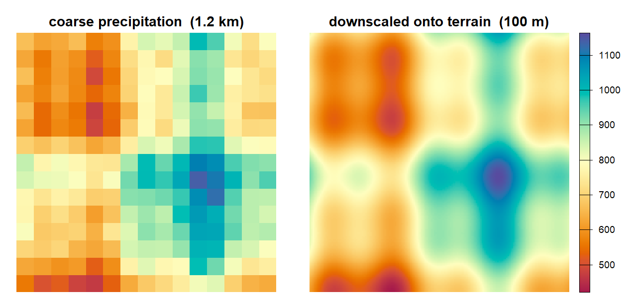
plot of chunk downscale
Give topocast a coarse variable and a fine predictor it
tracks. In a window around every cell it learns how the variable depends
on the predictor, then evaluates that local relationship on the fine
predictor. A 1 km precipitation grid and a 100 m elevation model become
a 100 m precipitation grid.
library(topocast)
library(terra)

names(prec_1km) <- "prec"      # coarse variable, what you want at high resolution
names(dem_100m) <- "elev"      # fine predictor it tracks

prec_100m <- topocast(prec ~ elev, data = prec_1km, onto = dem_100m, radius = 15)
prec_100m is precipitation on the elevation model’s
grid. Coarse to fine is one call: name the response and the predictor in
a formula, pass the coarse grid as data and the fine grid
as onto.
data is the coarse variable you want
at higher resolution, as a SpatRaster,
Raster*, or stars grid. The layer on the left
of the formula is the response.onto is the target: a fine grid
holding the predictor(s) the variable tracks, often a digital elevation
model. It can also be a set of station or plot points carrying those
predictors as attributes.onto, in the class of onto: a raster at the
fine resolution for a grid target, a prediction column for a point
target.When the only fine layer you have is the predictor itself, as in the
example above, topocast derives the coarse predictor from
onto for you, so a single coarse climate layer and a DEM
are enough to start.
The relationship is fit locally, in a square window around every
coarse cell, with summed-area tables: each window fit reduces to four
lookups per sufficient statistic, so a radius of 30 costs the same as a
radius of 3. The fitted intercept and slope grids are resampled to the
fine grid and combined with the fine predictors as
fitted = intercept + sum(slope * predictor), so the output
carries the fine-scale structure of the terrain with locally varying
coefficients. This is the regression step behind high-resolution climate
surfaces such as CHELSA (Karger et al. 2017); topocast runs
it locally and takes any number of named predictors.
topocast() takes a
formula, the coarse data, and the fine onto,
and returns the downscaled response.prec ~ elev + slope + twi fits elevation, slope,
topographic wetness, or any aligned covariate jointly. The formula names
match layers between data and onto, so a
missing layer is reported by name.cbind(prec, tmin) ~ elev downscales variables that share
the terrain together. The window design is built once and solved against
each response, so a second response costs little more than the
first.SpatRaster,
Raster* (raster), and stars grids are all
accepted; the result comes back in the class of onto, or
the class named by output.sf or
SpatVector of stations or plots as onto and
receive a prediction column, with the points carrying the fine predictor
values.anomaly to fit the baseline once and carry each period onto
it, "ratio" for precipitation or "additive"
for temperature.diagnostics = TRUE returns an r.squared grid
showing where the terrain relationship is strong, and
clamp = TRUE bounds the output to the observed range of the
coarse response.window_regression()
exposes the kernel for callers who hold their data as matrices.# install.packages("pak")
pak::pak("gcol33/topocast")Several predictors, matched by name between the two grids:
coarse <- c(prec_1km, elev_1km, twi_1km, slope_1km)
names(coarse) <- c("prec", "elev", "twi", "slope")
terrain <- c(elev_100m, twi_100m, slope_100m)
names(terrain) <- c("elev", "twi", "slope")

prec_100m <- topocast(prec ~ elev + twi + slope, data = coarse, onto = terrain,
                      radius = 15)
Several responses that share the terrain, downscaled in one pass and returned as one layer each:
climate_100m <- topocast(cbind(prec, tmin, tmax) ~ elev, data = coarse,
                         onto = terrain, radius = 15)
A monthly series sharing one terrain relationship across periods:
series <- topocast(prec ~ elev, data = coarse, onto = terrain, radius = 15,
                   anomaly = prec_monthly_1km, type = "ratio")
Downscaling straight to plot locations, returned as a column on the points:
at_plots <- topocast(prec ~ elev, data = coarse, onto = plots_sf, radius = 15)The local coefficient grids, to read the fitted lapse rate:
coefs <- topocast(prec ~ elev, data = coarse, onto = terrain, radius = 15,
coefficients = TRUE)“Software is like sex: it’s better when it’s free.” — Linus Torvalds
I’m a PhD student who builds R packages in my free time because I believe good tools should be free and open. I started these projects for my own work and figured others might find them useful too.
If this package saved you some time, buying me a coffee is a nice way to say thanks. It helps with my coffee addiction.
MIT. If you use topocast in published work, please cite
it:
@software{topocast,
  author = {Colling, Gilles},
  title  = {topocast: Moving-Window Regression Downscaling of Raster Data},
  year   = {2026},
  url    = {https://github.com/gcol33/topocast}
}
These binaries (installable software) and packages are in development.
They may not be fully stable and should be used with caution. We make no claims about them.
Health stats visible at Monitor.
