The hardware and bandwidth for this mirror is donated by dogado GmbH, the Webhosting and Full Service-Cloud Provider. Check out our Wordpress Tutorial.
If you wish to report a bug, or if you are interested in having us mirror your free-software or open-source project, please feel free to contact us at mirror[@]dogado.de.
![]()
![]()
Brings Seurat to the tidyverse!
website: stemangiola.github.io/tidyseurat/
Please also have a look at
tidyseurat provides a bridge between the Seurat single-cell package [@butler2018integrating; @stuart2019comprehensive] and the tidyverse [@wickham2019welcome]. It creates an invisible layer that enables viewing the Seurat object as a tidyverse tibble, and provides Seurat-compatible dplyr, tidyr, ggplot and plotly functions.
| Seurat-compatible Functions | Description |
|---|---|
all |
| tidyverse Packages | Description |
|---|---|
dplyr |
All dplyr APIs like for any tibble |
tidyr |
All tidyr APIs like for any tibble |
ggplot2 |
ggplot like for any tibble |
plotly |
plot_ly like for any tibble |
| Utilities | Description |
|---|---|
tidy |
Add tidyseurat invisible layer over a Seurat
object |
as_tibble |
Convert cell-wise information to a tbl_df |
join_features |
Add feature-wise information, returns a tbl_df |
aggregate_cells |
Aggregate cell gene-transcription abundance as pseudobulk tissue |
From CRAN
install.packages("tidyseurat")From Github (development)
devtools::install_github("stemangiola/tidyseurat")library(dplyr)
library(tidyr)
library(purrr)
library(magrittr)
library(ggplot2)
library(Seurat)
library(tidyseurat)tidyseurat, the best of both worlds!This is a seurat object but it is evaluated as tibble. So it is fully compatible both with Seurat and tidyverse APIs.
pbmc_small = SeuratObject::pbmc_smallIt looks like a tibble
pbmc_small## # A Seurat-tibble abstraction: 80 × 15
## # [90mFeatures=230 | Cells=80 | Active assay=RNA | Assays=RNA[0m
## .cell orig.ident nCount_RNA nFeature_RNA RNA_snn_res.0.8 letter.idents groups
## <chr> <fct> <dbl> <int> <fct> <fct> <chr>
## 1 ATGC… SeuratPro… 70 47 0 A g2
## 2 CATG… SeuratPro… 85 52 0 A g1
## 3 GAAC… SeuratPro… 87 50 1 B g2
## 4 TGAC… SeuratPro… 127 56 0 A g2
## 5 AGTC… SeuratPro… 173 53 0 A g2
## 6 TCTG… SeuratPro… 70 48 0 A g1
## 7 TGGT… SeuratPro… 64 36 0 A g1
## 8 GCAG… SeuratPro… 72 45 0 A g1
## 9 GATA… SeuratPro… 52 36 0 A g1
## 10 AATG… SeuratPro… 100 41 0 A g1
## # ℹ 70 more rows
## # ℹ 8 more variables: RNA_snn_res.1 <fct>, PC_1 <dbl>, PC_2 <dbl>, PC_3 <dbl>,
## # PC_4 <dbl>, PC_5 <dbl>, tSNE_1 <dbl>, tSNE_2 <dbl>But it is a Seurat object after all
pbmc_small@assays## $RNA
## Assay data with 230 features for 80 cells
## Top 10 variable features:
## PPBP, IGLL5, VDAC3, CD1C, AKR1C3, PF4, MYL9, GNLY, TREML1, CA2Set colours and theme for plots.
# Use colourblind-friendly colours
friendly_cols <- c("#88CCEE", "#CC6677", "#DDCC77", "#117733", "#332288", "#AA4499", "#44AA99", "#999933", "#882255", "#661100", "#6699CC")

# Set theme
my_theme <-
  list(
    scale_fill_manual(values = friendly_cols),
    scale_color_manual(values = friendly_cols),
    theme_bw() +
      theme(
        panel.border = element_blank(),
        axis.line = element_line(),
        panel.grid.major = element_line(size = 0.2),
        panel.grid.minor = element_line(size = 0.1),
        text = element_text(size = 12),
        legend.position = "bottom",
        aspect.ratio = 1,
        strip.background = element_blank(),
        axis.title.x = element_text(margin = margin(t = 10, r = 10, b = 10, l = 10)),
        axis.title.y = element_text(margin = margin(t = 10, r = 10, b = 10, l = 10))
      )
  )
We can treat pbmc_small effectively as a normal tibble
for plotting.
Here we plot number of features per cell.
pbmc_small %>%
  ggplot(aes(nFeature_RNA, fill = groups)) +
  geom_histogram() +
  my_theme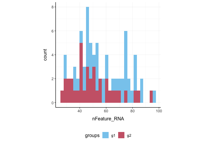
Here we plot total features per cell.
pbmc_small %>%
  ggplot(aes(groups, nCount_RNA, fill = groups)) +
  geom_boxplot(outlier.shape = NA) +
  geom_jitter(width = 0.1) +
  my_theme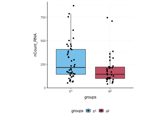
Here we plot abundance of two features for each group.
pbmc_small %>%
  join_features(features = c("HLA-DRA", "LYZ"), shape = "long") %>%
  ggplot(aes(groups, .abundance_RNA + 1, fill = groups)) +
  geom_boxplot(outlier.shape = NA) +
  geom_jitter(aes(size = nCount_RNA), alpha = 0.5, width = 0.2) +
  scale_y_log10() +
  my_theme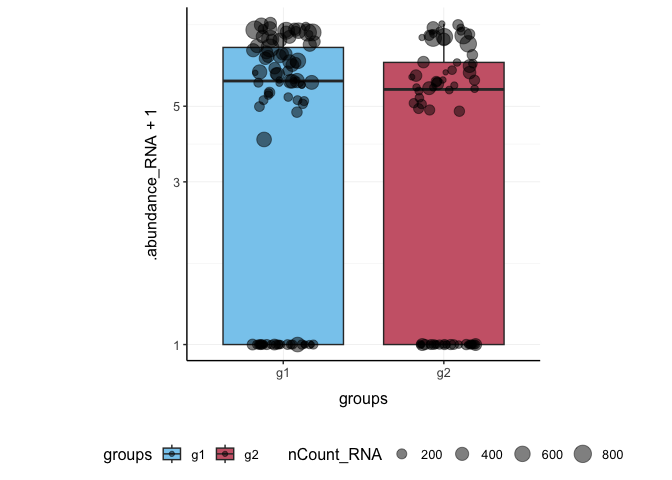
Also you can treat the object as Seurat object and proceed with data processing.
pbmc_small_pca <-
  pbmc_small %>%
  SCTransform(verbose = FALSE) %>%
  FindVariableFeatures(verbose = FALSE) %>%
  RunPCA(verbose = FALSE)

pbmc_small_pca
## # A Seurat-tibble abstraction: 80 × 17
## # [90mFeatures=220 | Cells=80 | Active assay=SCT | Assays=RNA, SCT[0m
## .cell orig.ident nCount_RNA nFeature_RNA RNA_snn_res.0.8 letter.idents groups
## <chr> <fct> <dbl> <int> <fct> <fct> <chr>
## 1 ATGC… SeuratPro… 70 47 0 A g2
## 2 CATG… SeuratPro… 85 52 0 A g1
## 3 GAAC… SeuratPro… 87 50 1 B g2
## 4 TGAC… SeuratPro… 127 56 0 A g2
## 5 AGTC… SeuratPro… 173 53 0 A g2
## 6 TCTG… SeuratPro… 70 48 0 A g1
## 7 TGGT… SeuratPro… 64 36 0 A g1
## 8 GCAG… SeuratPro… 72 45 0 A g1
## 9 GATA… SeuratPro… 52 36 0 A g1
## 10 AATG… SeuratPro… 100 41 0 A g1
## # ℹ 70 more rows
## # ℹ 10 more variables: RNA_snn_res.1 <fct>, nCount_SCT <dbl>,
## # nFeature_SCT <int>, PC_1 <dbl>, PC_2 <dbl>, PC_3 <dbl>, PC_4 <dbl>,
## # PC_5 <dbl>, tSNE_1 <dbl>, tSNE_2 <dbl>If a tool is not included in the tidyseurat collection, we can use
as_tibble to permanently convert tidyseurat
into tibble.
pbmc_small_pca %>%
  as_tibble() %>%
  select(contains("PC"), everything()) %>%
  GGally::ggpairs(columns = 1:5, ggplot2::aes(colour = groups)) +
  my_theme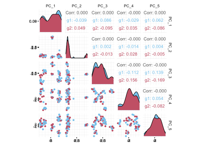
We proceed with cluster identification with Seurat.
pbmc_small_cluster <-
  pbmc_small_pca %>%
  FindNeighbors(verbose = FALSE) %>%
  FindClusters(method = "igraph", verbose = FALSE)

pbmc_small_cluster
## # A Seurat-tibble abstraction: 80 × 19
## # [90mFeatures=220 | Cells=80 | Active assay=SCT | Assays=RNA, SCT[0m
## .cell orig.ident nCount_RNA nFeature_RNA RNA_snn_res.0.8 letter.idents groups
## <chr> <fct> <dbl> <int> <fct> <fct> <chr>
## 1 ATGC… SeuratPro… 70 47 0 A g2
## 2 CATG… SeuratPro… 85 52 0 A g1
## 3 GAAC… SeuratPro… 87 50 1 B g2
## 4 TGAC… SeuratPro… 127 56 0 A g2
## 5 AGTC… SeuratPro… 173 53 0 A g2
## 6 TCTG… SeuratPro… 70 48 0 A g1
## 7 TGGT… SeuratPro… 64 36 0 A g1
## 8 GCAG… SeuratPro… 72 45 0 A g1
## 9 GATA… SeuratPro… 52 36 0 A g1
## 10 AATG… SeuratPro… 100 41 0 A g1
## # ℹ 70 more rows
## # ℹ 12 more variables: RNA_snn_res.1 <fct>, nCount_SCT <dbl>,
## # nFeature_SCT <int>, SCT_snn_res.0.8 <fct>, seurat_clusters <fct>,
## # PC_1 <dbl>, PC_2 <dbl>, PC_3 <dbl>, PC_4 <dbl>, PC_5 <dbl>, tSNE_1 <dbl>,
## # tSNE_2 <dbl>Now we can interrogate the object as if it was a regular tibble data frame.
pbmc_small_cluster %>%
  count(groups, seurat_clusters)
## # A tibble: 6 × 3
## groups seurat_clusters n
## <chr> <fct> <int>
## 1 g1 0 23
## 2 g1 1 17
## 3 g1 2 4
## 4 g2 0 17
## 5 g2 1 13
## 6 g2 2 6We can identify cluster markers using Seurat.
# Identify top 10 markers per cluster
markers <-
  pbmc_small_cluster %>%
  FindAllMarkers(only.pos = TRUE, min.pct = 0.25, thresh.use = 0.25) %>%
  group_by(cluster) %>%
  top_n(10, avg_log2FC)

# Plot heatmap
pbmc_small_cluster %>%
  DoHeatmap(
    features = markers$gene,
    group.colors = friendly_cols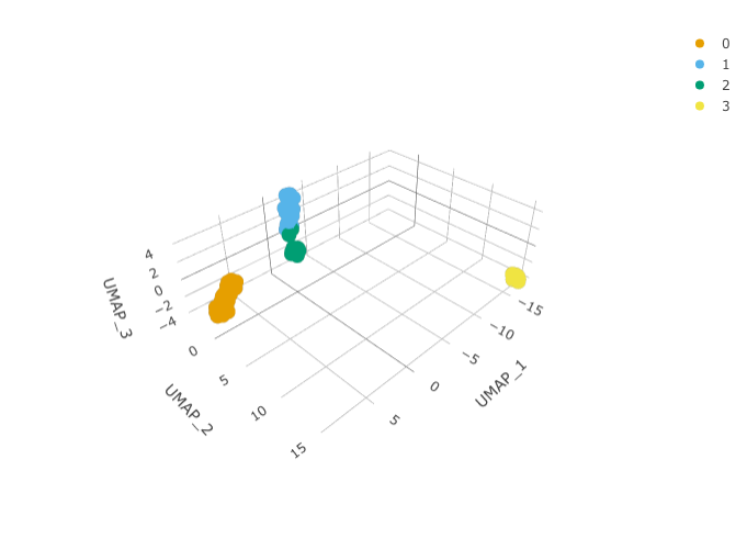
)We can calculate the first 3 UMAP dimensions using the Seurat framework.
pbmc_small_UMAP <-
  pbmc_small_cluster %>%
  RunUMAP(reduction = "pca", dims = 1:15, n.components = 3L)
And we can plot them using 3D plot using plotly.
pbmc_small_UMAP %>%
  plot_ly(
    x = ~`UMAP_1`,
    y = ~`UMAP_2`,
    z = ~`UMAP_3`,
    color = ~seurat_clusters,
    colors = friendly_cols[1:4]
  )
We can infer cell type identities using SingleR [@aran2019reference] and manipulate the output using tidyverse.
# Get cell type reference data
blueprint <- celldex::BlueprintEncodeData()

# Infer cell identities
cell_type_df <-
  GetAssayData(pbmc_small_UMAP, slot = 'counts', assay = "SCT") %>%
  log1p() %>%
  Matrix::Matrix(sparse = TRUE) %>%
  SingleR::SingleR(
    ref = blueprint,
    labels = blueprint$label.main,
    method = "single"
  ) %>%
  as.data.frame() %>%
  as_tibble(rownames = "cell") %>%
  select(cell, first.labels)
# Join UMAP and cell type info
pbmc_small_cell_type <-
pbmc_small_UMAP %>%
left_join(cell_type_df, by = "cell")
# Reorder columns
pbmc_small_cell_type %>%
select(cell, first.labels, everything())We can easily summarise the results. For example, we can see how cell type classification overlaps with cluster classification.
pbmc_small_cell_type %>%
  count(seurat_clusters, first.labels)
We can easily reshape the data for building information-rich faceted plots.
pbmc_small_cell_type %>%

  # Reshape and add classifier column
  pivot_longer(
    cols = c(seurat_clusters, first.labels),
    names_to = "classifier", values_to = "label"
  ) %>%

  # UMAP plots for cell type and cluster
  ggplot(aes(UMAP_1, UMAP_2, color = label)) +
  geom_point() +
  facet_wrap(~classifier) +
  my_theme
We can easily plot gene correlation per cell category, adding multi-layer annotations.
pbmc_small_cell_type %>%

  # Add some mitochondrial abundance values
  mutate(mitochondrial = rnorm(n())) %>%

  # Plot correlation
  join_features(features = c("CST3", "LYZ"), shape = "wide") %>%
  ggplot(aes(CST3 + 1, LYZ + 1, color = groups, size = mitochondrial)) +
  geom_point() +
  facet_wrap(~first.labels, scales = "free") +
  scale_x_log10() +
  scale_y_log10() +
my_themeA powerful tool we can use with tidyseurat is nest. We
can easily perform independent analyses on subsets of the dataset. First
we classify cell types in lymphoid and myeloid; then, nest based on the
new classification
pbmc_small_nested <-
  pbmc_small_cell_type %>%
  filter(first.labels != "Erythrocytes") %>%
  mutate(cell_class = if_else(`first.labels` %in% c("Macrophages", "Monocytes"), "myeloid", "lymphoid")) %>%
  nest(data = -cell_class)

pbmc_small_nested
Now we can independently for the lymphoid and myeloid subsets (i) find variable features, (ii) reduce dimensions, and (iii) cluster using both tidyverse and Seurat seamlessly.
pbmc_small_nested_reanalysed <-
  pbmc_small_nested %>%
  mutate(data = map(
    data, ~ .x %>%
      FindVariableFeatures(verbose = FALSE) %>%
      RunPCA(npcs = 10, verbose = FALSE) %>%
      FindNeighbors(verbose = FALSE) %>%
      FindClusters(method = "igraph", verbose = FALSE) %>%
      RunUMAP(reduction = "pca", dims = 1:10, n.components = 3L, verbose = FALSE)
  ))

pbmc_small_nested_reanalysed
Now we can unnest and plot the new classification.
pbmc_small_nested_reanalysed %>%

  # Convert to tibble otherwise Seurat drops reduced dimensions when unifying data sets.
  mutate(data = map(data, ~ .x %>% as_tibble())) %>%
  unnest(data) %>%

  # Define unique clusters
  unite("cluster", c(cell_class, seurat_clusters), remove = FALSE) %>%

  # Plotting
  ggplot(aes(UMAP_1, UMAP_2, color = cluster)) +
  geom_point() +
  facet_wrap(~cell_class) +
my_themeSometimes, it is necessary to aggregate the gene-transcript abundance from a group of cells into a single value. For example, when comparing groups of cells across different samples with fixed-effect models.
In tidyseurat, cell aggregation can be achieved using the
aggregate_cells function.
pbmc_small %>%
  aggregate_cells(groups, assays = "RNA")
These binaries (installable software) and packages are in development.
They may not be fully stable and should be used with caution. We make no claims about them.
Health stats visible at Monitor.