The hardware and bandwidth for this mirror is donated by dogado GmbH, the Webhosting and Full Service-Cloud Provider. Check out our Wordpress Tutorial.
If you wish to report a bug, or if you are interested in having us mirror your free-software or open-source project, please feel free to contact us at mirror[@]dogado.de.
![]()
Monte Carlo Simulations aim to study the properties of statistical
inference techniques. At its core, a Monte Carlo Simulation works
through the application of the techniques to repeatedly drawn samples
from a pre-specified data generating process. The tidyMC
package aims to cover and simplify the whole workflow of running a Monte
Carlo simulation in either an academic or professional setting. Thus,
tidyMC aims to provide functions for the following
tasks:
future_mc()summary.mc()plot.mc() and
plot.summary.mc()LaTeX table summarizing the results of the
Monte Carlo Simulation using tidy_mc_latex()Install from CRAN
install.packages("tidyMC")or download the development version from GitHub as follows:
# install.packages("devtools")
devtools::install_github("stefanlinner/tidyMC", build_vignettes = TRUE)
Afterwards you can load the package:
library(tidyMC)library(magrittr)
library(ggplot2)
library(kableExtra)This is a basic example which shows you how to solve a common problem. For a more elaborate example please see the vignette:
browseVignettes(package = "tidyMC")
#> starte den http Server für die Hilfe fertig
Run your first Monte Carlo Simulation using your own parameter grid:
test_func <- function(param = 0.1, n = 100, x1 = 1, x2 = 2){

  data <- rnorm(n, mean = param) + x1 + x2
  stat <- mean(data)
  stat_2 <- var(data)

  if (x2 == 5){
    stop("x2 can't be 5!")
  }

  return(list(mean = stat, var = stat_2))
}

param_list <- list(param = seq(from = 0, to = 1, by = 0.5),
                   x1 = 1:2)

set.seed(101)

test_mc <- future_mc(
  fun = test_func,
  repetitions = 1000,
  param_list = param_list,
  n = 10,
  x2 = 2,
  check = TRUE
)
#> Running single test-iteration for each parameter combination...
#>
#>  Test-run successfull: No errors occurred!
#> Running whole simulation: Overall 6 parameter combinations are simulated ...
#>
#>  Simulation was successfull!
#>  Running time: 00:00:06.505337

test_mc
#> Monte Carlo simulation results for the specified function:
#>
#>  function (param = 0.1, n = 100, x1 = 1, x2 = 2)
#> {
#>     data <- rnorm(n, mean = param) + x1 + x2
#>     stat <- mean(data)
#>     stat_2 <- var(data)
#>     if (x2 == 5) {
#>         stop("x2 can't be 5!")
#>     }
#>     return(list(mean = stat, var = stat_2))
#> }
#>
#>  The following 6 parameter combinations:
#> # A tibble: 6 × 2
#>   param    x1
#>   <dbl> <int>
#> 1   0       1
#> 2   0.5     1
#> 3   1       1
#> 4   0       2
#> 5   0.5     2
#> 6   1       2
#> are each simulated 1000 times.
#>
#>  The Running time was: 00:00:06.505337
#>
#>  Parallel: TRUE
#>
#>  The following parallelisation plan was used:
#> $strategy
#> multisession:
#> - args: function (..., workers = availableCores(), lazy = FALSE, rscript_libs = .libPaths(), envir = parent.frame())
#> - tweaked: FALSE
#> - call: NULL
#>
#>
#>  Seed: TRUE
Summarize your results:
sum_res <- summary(test_mc)
sum_res
#> Results for the output mean:
#>    param=0, x1=1: 3.015575
#>    param=0, x1=2: 4.003162
#>    param=0.5, x1=1: 3.49393
#>    param=0.5, x1=2: 4.480855
#>    param=1, x1=1: 3.985815
#>    param=1, x1=2: 4.994084
#>
#>
#> Results for the output var:
#>    param=0, x1=1: 0.9968712
#>    param=0, x1=2: 1.026523
#>    param=0.5, x1=1: 0.9933278
#>    param=0.5, x1=2: 0.9997529
#>    param=1, x1=1: 0.9979682
#>    param=1, x1=2: 1.005633
#>
#>
Plot your results / summarized results:
returned_plot1 <- plot(test_mc, plot = FALSE)

returned_plot1$mean +
 ggplot2::theme_minimal() +
 ggplot2::geom_vline(xintercept = 3)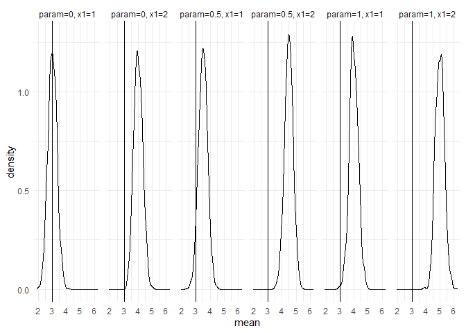
returned_plot2 <- plot(test_mc, which_setup = test_mc$nice_names[1:2], plot = FALSE)
returned_plot2$mean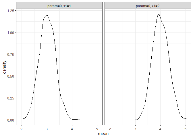
returned_plot3 <- plot(test_mc, join = test_mc$nice_names[1:2], plot = FALSE)
returned_plot3$mean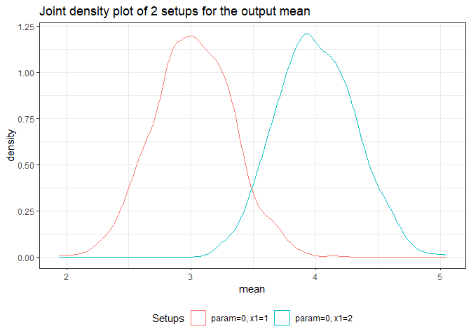
returned_plot1 <- plot(summary(test_mc), plot = FALSE)

returned_plot1$mean +
  ggplot2::theme_minimal()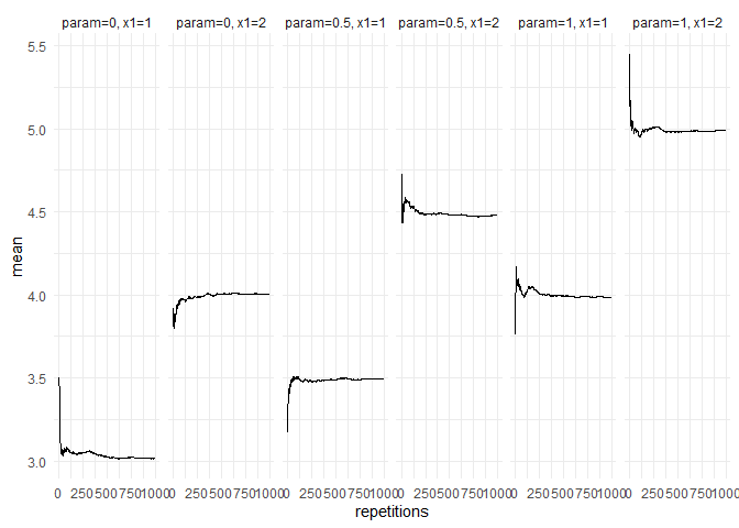
returned_plot2 <- plot(summary(test_mc), which_setup = test_mc$nice_names[1:2], plot = FALSE)
 returned_plot2$mean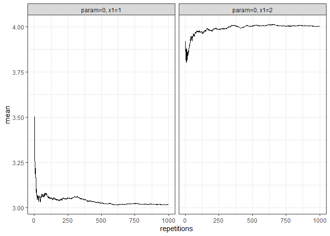
returned_plot3 <- plot(summary(test_mc), join = test_mc$nice_names[1:2], plot = FALSE)
returned_plot3$mean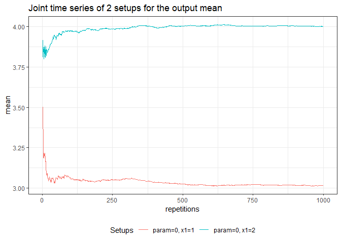
Show your results in a LaTeX table:
tidy_mc_latex(summary(test_mc)) %>%
  print()
#> \begin{table}
#>
#> \caption{\label{tab:unnamed-chunk-10}Monte Carlo simulations results}
#> \centering
#> \begin{tabular}[t]{cccc}
#> \toprule
#> param & x1 & mean & var\\
#> \midrule
#> 0.0 & 1 & 3.016 & 0.997\\
#> 0.0 & 2 & 4.003 & 1.027\\
#> 0.5 & 1 & 3.494 & 0.993\\
#> 0.5 & 2 & 4.481 & 1.000\\
#> 1.0 & 1 & 3.986 & 0.998\\
#> \addlinespace
#> 1.0 & 2 & 4.994 & 1.006\\
#> \bottomrule
#> \multicolumn{4}{l}{\textsuperscript{} Total repetitions = 1000,}\\
#> \multicolumn{4}{l}{total parameter combinations}\\
#> \multicolumn{4}{l}{= 6}\\
#> \end{tabular}
#> \end{table}

tidy_mc_latex(
    summary(test_mc),
    repetitions_set = c(10,1000),
    which_out = "mean",
    kable_options = list(caption = "Mean MCS results")
) %>%
  print()
#> \begin{table}
#>
#> \caption{\label{tab:unnamed-chunk-10}Mean MCS results}
#> \centering
#> \begin{tabular}[t]{ccc}
#> \toprule
#> param & x1 & mean\\
#> \midrule
#> \addlinespace[0.3em]
#> \multicolumn{3}{l}{\textbf{N = 10}}\\
#> \hspace{1em}0.0 & 1 & 3.193\\
#> \hspace{1em}0.0 & 2 & 3.810\\
#> \hspace{1em}0.5 & 1 & 3.434\\
#> \hspace{1em}0.5 & 2 & 4.550\\
#> \hspace{1em}1.0 & 1 & 4.156\\
#> \hspace{1em}1.0 & 2 & 5.030\\
#> \addlinespace[0.3em]
#> \multicolumn{3}{l}{\textbf{N = 1000}}\\
#> \hspace{1em}0.0 & 1 & 3.016\\
#> \hspace{1em}0.0 & 2 & 4.003\\
#> \hspace{1em}0.5 & 1 & 3.494\\
#> \hspace{1em}0.5 & 2 & 4.481\\
#> \hspace{1em}1.0 & 1 & 3.986\\
#> \hspace{1em}1.0 & 2 & 4.994\\
#> \bottomrule
#> \multicolumn{3}{l}{\textsuperscript{} Total repetitions =}\\
#> \multicolumn{3}{l}{1000, total}\\
#> \multicolumn{3}{l}{parameter}\\
#> \multicolumn{3}{l}{combinations = 6}\\
#> \end{tabular}
#> \end{table}
These binaries (installable software) and packages are in development.
They may not be fully stable and should be used with caution. We make no claims about them.
Health stats visible at Monitor.