The hardware and bandwidth for this mirror is donated by dogado GmbH, the Webhosting and Full Service-Cloud Provider. Check out our Wordpress Tutorial.
If you wish to report a bug, or if you are interested in having us mirror your free-software or open-source project, please feel free to contact us at mirror[@]dogado.de.
Differential analysis of tumor tissue immune cell type abundance based on RNASeq gene-level expression from The Cancer Genome Atlas (TCGA) database.
Required: - Softwares : R (≥ 3.3.0); RStudio (https://posit.co/downloads/) - R libraries : see the DESCRIPTION file.
You can install the development version from GitHub with:
# install.packages("devtools")
devtools::install_github("ecamenen/tcgaViz")system.file("extdata", package = "tcgaViz").tcgaViz::run_app()docker pull eucee/tcga-vizdocker run --rm -p 127.0.0.1:3838:3838 eucee/tcga-vizA subset of invasive breast carcinoma data from primary tumor tissue.
See ?tcga for more information on loading the full dataset
or metadata.
library(tcgaViz)
library(ggplot2)
data(tcga)
head(tcga$genes)
#> # A tibble: 6 x 2
#>   sample           ICOS
#>   <chr>           <dbl>
#> 1 TCGA-3C-AAAU-01  1.25
#> 2 TCGA-A2-A04Q-01  7.79
#> 3 TCGA-A2-A0T4-01  4.97
#> 4 TCGA-A8-A08S-01  3.69
#> 5 TCGA-A8-A09B-01  2.55
#> 6 TCGA-A8-A0AD-01  3.72
head(tcga$cells$Cibersort_ABS)
#> # A tibble: 6 x 24
#>   sample          study B_cell_naive B_cell_memory B_cell_plasma T_cell_CD8.
#>   <chr>           <fct>        <dbl>         <dbl>         <dbl>       <dbl>
#> 1 TCGA-3C-AAAU-01 BRCA      0             0.0221         0.0192       0.0129
#> 2 TCGA-A2-A04Q-01 BRCA      0.0274        0.0249         0.0236       0.118
#> 3 TCGA-A2-A0T4-01 BRCA      0.0167        0              0.0159       0.0432
#> 4 TCGA-A8-A08S-01 BRCA      0             0.00425        0            0.0217
#> 5 TCGA-A8-A09B-01 BRCA      0.0146        0              0.00612      0.0256
#> 6 TCGA-A8-A0AD-01 BRCA      0.000919      0.000797       0.00290      0
#> # … with 18 more variables: T_cell_CD4._naive <dbl>,
#> #   T_cell_CD4._memory_resting <dbl>, T_cell_CD4._memory_activated <dbl>,
#> #   T_cell_follicular_helper <dbl>, T_cell_regulatory_.Tregs. <dbl>,
#> #   T_cell_gamma_delta <dbl>, NK_cell_resting <dbl>, NK_cell_activated <dbl>,
#> #   Monocyte <dbl>, Macrophage_M0 <dbl>, Macrophage_M1 <dbl>,
#> #   Macrophage_M2 <dbl>, Myeloid_dendritic_cell_resting <dbl>,
#> #   Myeloid_dendritic_cell_activated <dbl>, Mast_cell_activated <dbl>,
#> # Mast_cell_resting <dbl>, Eosinophil <dbl>, Neutrophil <dbl>And perform a significance of a Wilcoxon adjusted test according to the expression level (high or low) of a selected gene.
(df <- convert2biodata(
  algorithm = "Cibersort_ABS",
  disease = "breast invasive carcinoma",
  tissue = "Primary Tumor",
  gene_x = "ICOS"
))
#> # A tibble: 660 x 3
#>    high  cell_type       value
#>  * <fct> <fct>           <dbl>
#>  1 Low   B_cell_naive 0.00001
#>  2 High  B_cell_naive 0.0274
#>  3 High  B_cell_naive 0.0167
#>  4 Low   B_cell_naive 0.00001
#>  5 Low   B_cell_naive 0.0146
#>  6 Low   B_cell_naive 0.000929
#>  7 Low   B_cell_naive 0.00180
#>  8 High  B_cell_naive 0.0112
#>  9 Low   B_cell_naive 0.0141
#> 10 Low   B_cell_naive 0.00546
#> # … with 650 more rows
(stats <- calculate_pvalue(df))
#> Breast Invasive Carcinoma (BRCA; Primary Tumor)
#> Wilcoxon-Mann-Whitney test with Benjamini & Hochberg correction (n_low = 16; n_high = 14).
#> # A tibble: 6 x 9
#>   `Cell type`                `Average(High)` `Average(Low)` `SD(High)` `SD(Low)`
#>   <fct>                                <dbl>          <dbl>      <dbl>     <dbl>
#> 1 Macrophage_M1                      0.0454        0.00943      0.0328   0.0116
#> 2 Macrophage_M2                      0.109         0.0697       0.0321   0.0368
#> 3 T_cell_CD4._memory_resting         0.0504        0.0122       0.0377   0.0124
#> 4 T_cell_CD8.                        0.0498        0.0127       0.0387   0.00934
#> 5 T_cell_follicular_helper           0.0352        0.0119       0.0259   0.00691
#> 6 T_cell_gamma_delta                 0.00823       0.000956     0.0101   0.00258
#> # … with 4 more variables: Average(High - Low) <dbl>, P-value <dbl>,
#> #   P-value adjusted <dbl>, Significance <chr>
plot(df, stats = stats)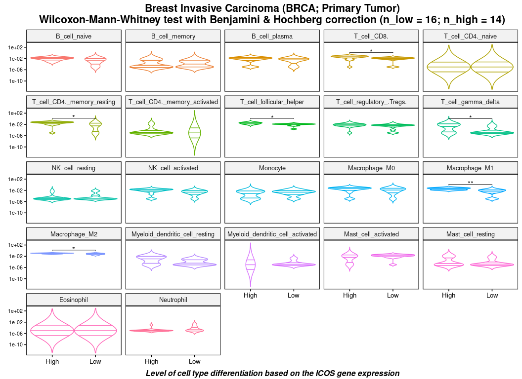
With ggplot2::theme() expressions.
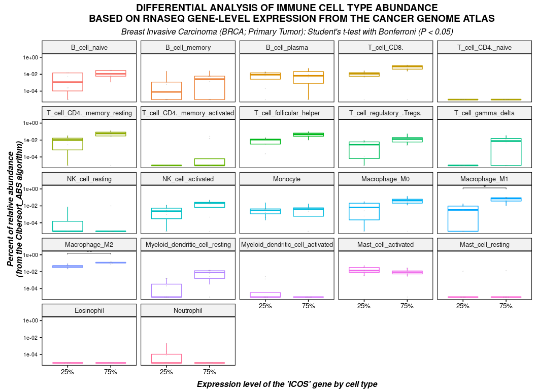
(df <- convert2biodata(
  algorithm = "Cibersort_ABS",
  disease = "breast invasive carcinoma",
  tissue = "Primary Tumor",
  gene_x = "ICOS",
  stat = "quantile"
))
#> # A tibble: 352 x 3
#>    high  cell_type      value
#>  * <fct> <fct>          <dbl>
#>  1 25%   B_cell_naive 0.00001
#>  2 75%   B_cell_naive 0.0274
#>  3 25%   B_cell_naive 0.0146
#>  4 75%   B_cell_naive 0.0112
#>  5 25%   B_cell_naive 0.0141
#>  6 25%   B_cell_naive 0.00546
#>  7 75%   B_cell_naive 0.0289
#>  8 75%   B_cell_naive 0.00376
#>  9 25%   B_cell_naive 0.00001
#> 10 75%   B_cell_naive 0.00118
#> # … with 342 more rows
(stats <- calculate_pvalue(
    df,
    method_test = "t_test",
    method_adjust = "bonferroni",
    p_threshold = 0.05
))
#> Breast Invasive Carcinoma (BRCA; Primary Tumor)
#> Student's t-test with bonferroni correction (n_low = 8; n_high = 8).
#> # A tibble: 2 x 9
#>   `Cell type` `Average(75%)` `Average(25%)` `SD(75%)` `SD(25%)` `Average(75% - …
#>   <fct>                <dbl>          <dbl>     <dbl>     <dbl>            <dbl>
#> 1 Macrophage…         0.0646        0.00560    0.0348   0.00651           0.0590
#> 2 Macrophage…         0.117         0.0456     0.0274   0.0216            0.0719
#> # … with 3 more variables: P-value <dbl>, P-value adjusted <dbl>,
#> #   Significance <chr>
plot(
    df,
    stats = stats,
    type = "boxplot",
    dots = TRUE,
    xlab = "Expression level of the 'ICOS' gene by cell type",
    ylab = "Percent of relative abundance\n(from the Cibersort_ABS algorithm)",
    title = toupper("Differential analysis of immune cell type abundance
    based on RNASeq gene-level expression from The Cancer Genome Atlas"),
    axis.text.y = element_text(size = 8, hjust = 0.5),
    plot.title =  element_text(face = "bold", hjust = 0.5),
    plot.subtitle =  element_text(size = , face = "italic", hjust = 0.5),
    draw = FALSE
) + labs(
    subtitle = paste("Breast Invasive Carcinoma (BRCA; Primary Tumor):",
    "Student's t-test with Bonferroni (P < 0.05)")
)
These binaries (installable software) and packages are in development.
They may not be fully stable and should be used with caution. We make no claims about them.
Health stats visible at Monitor.