The hardware and bandwidth for this mirror is donated by dogado GmbH, the Webhosting and Full Service-Cloud Provider. Check out our Wordpress Tutorial.
If you wish to report a bug, or if you are interested in having us mirror your free-software or open-source project, please feel free to contact us at mirror[@]dogado.de.

Surveyexplorer

Visualize and tabulate single-choice, multiple-choice, matrix-style questions from survey data. Includes ability to group cross-tabulations, frequency distributions, and plots by categorical variables and to integrate survey weights. Ideal for quickly uncovering descriptive patterns in survey data.

Installation

install.packages("surveyexplorer")
# or devtools::install_github("liamhaller/surveyexplorer") for the devlopment version 

Examples

library(surveyexplorer)

The data used in the following examples is from the berlinbears dataset, a fictional survey of bears in Berlin, that is included in the surveyexplorer package.

Single-choice questions

#Basic table
single_table(berlinbears, 
             question = income)

Use group_by = to partition the question into several groups

single_table(berlinbears,
             question = income,
             group_by = gender)

Ignore unwanted subgroups with subgroups_to_exclude

single_table(berlinbears,
             question = income, 
             group_by = gender, 
             subgroups_to_exclude = NA) 

Remove NAs from the question variable with na.rm

single_table(berlinbears,
             question = income, 
             group_by = gender, 
             subgroups_to_exclude = NA,
             na.rm = TRUE)

Finally, you can specify survey weights using the weight option

single_table(berlinbears,
             question = income, 
             group_by = gender, 
             subgroups_to_exclude = NA,
             na.rm = TRUE,
             weights = weights)

The same syntax can be applied to the single_freq function to plot frequencies of the question optionally partitioned by subgroups.

single_freq(berlinbears,
             question = income, 
             group_by = gender, 
             subgroups_to_exclude = NA,
             na.rm = TRUE,
             weights = weights)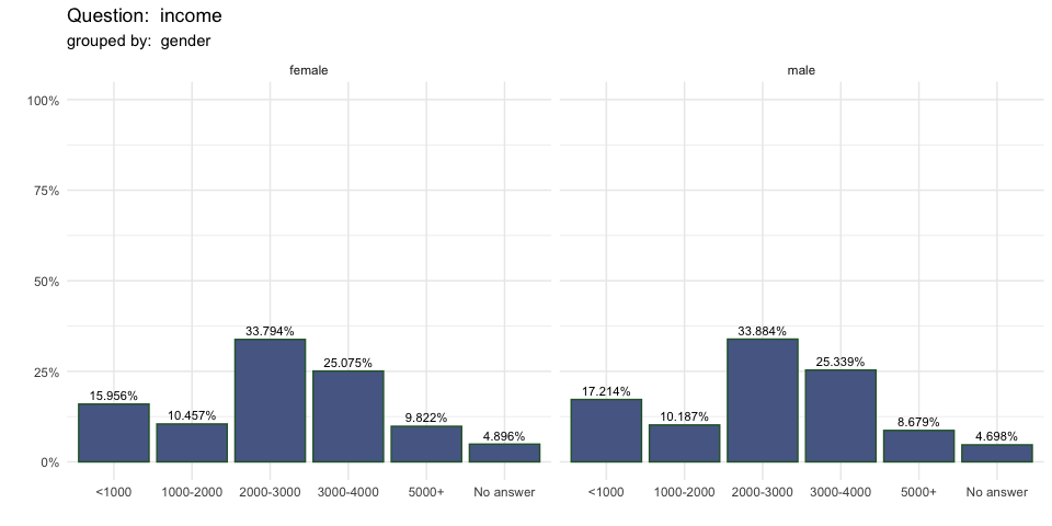

Multiple-choice questions

The options and syntax for multiple-choice tables multi_table and graphs multi_graphs are the same. The only difference is the question input also accommodates tidyselect syntax to select several columns for each answer option. For example, the question “will_eat” has five answer options each prefixed by “will_eat”

berlinbears |> 
  dplyr::select(starts_with('will_eat')) |> 
  head()
#>   will_eat.SQ001 will_eat.SQ002 will_eat.SQ003 will_eat.SQ004 will_eat.SQ005
#> 1              0              1              0              1              1
#> 2              0              1              1              1              1
#> 3              1              1              0              1              1
#> 4              0              0              0              1              0
#> 5              0              0              0              1              1
#> 6              0              0              0              1              0

The same syntax can be used to select the question for the multiple choice tables and graphs

multi_table(berlinbears, 
            question = dplyr::starts_with('will_eat'), 
            group_by = genus, 
            subgroups_to_exclude = NA,
            na.rm = TRUE)

For graphing, the multi_freq function creates an UpSet plot to visualize the frequencies of the intersecting sets for each answer combination and also includes the ability to specify weights.

multi_freq(berlinbears, 
            question = dplyr::starts_with('will_eat'), 
            na.rm = TRUE,
            weights = weights)
#> Estimes are only preciese to one significant digit, weights may have been rounded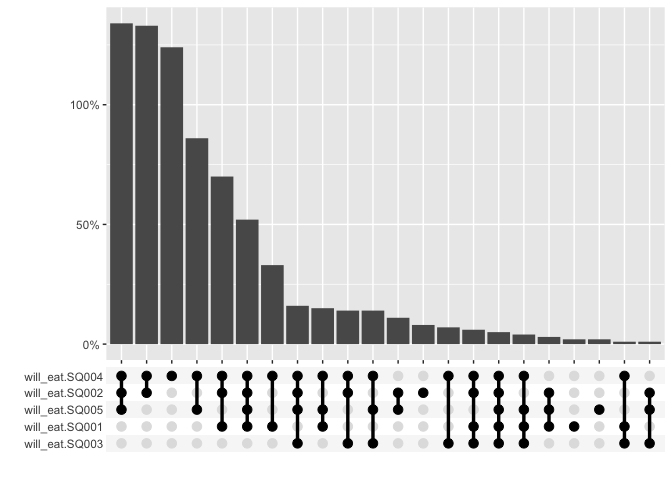

The graphs can also be grouped

multi_freq(berlinbears, 
            question = dplyr::starts_with('will_eat'), 
            group_by = genus,
            subgroups_to_exclude = NA,
            na.rm = FALSE,
            weights = weights)
#> Estimes are only preciese to one significant digit, weights may have been rounded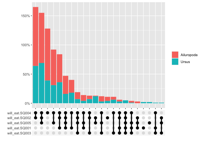

Matrix Questions

matrix_table has the same syntax as above and works with array or categorical questions

matrix_table(berlinbears, 
             dplyr::starts_with('c_'),
             group_by = is_parent)

matrix_freq visualizes the frequencies of responses

matrix_freq(berlinbears, 
             dplyr::starts_with('p_'), 
             na.rm = TRUE)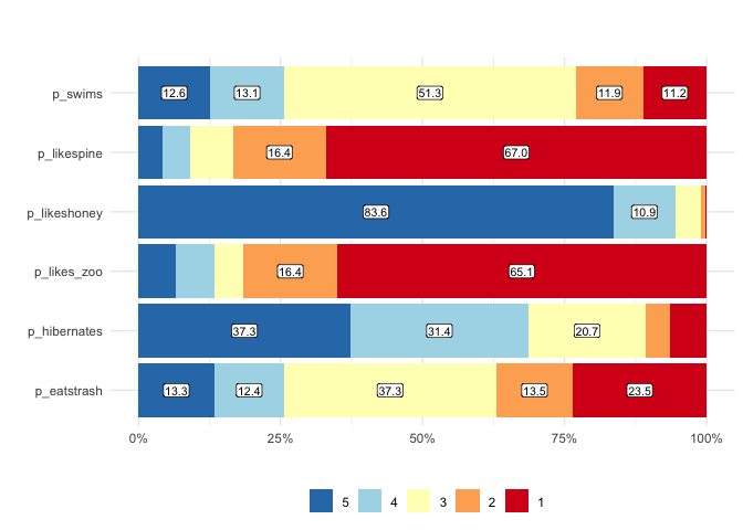

For array/matrix style questions that are numeric matrix_mean plots the mean values and confidence intervals

matrix_mean(berlinbears, 
             question = dplyr::starts_with('p_'),
             na.rm = TRUE)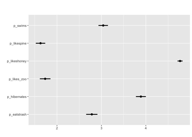

#Can also apply grouping + survey weights
matrix_mean(berlinbears, 
            question = dplyr::starts_with('p_'),
            na.rm = TRUE,
            group_by = species, 
            subgroups_to_exclude = NA)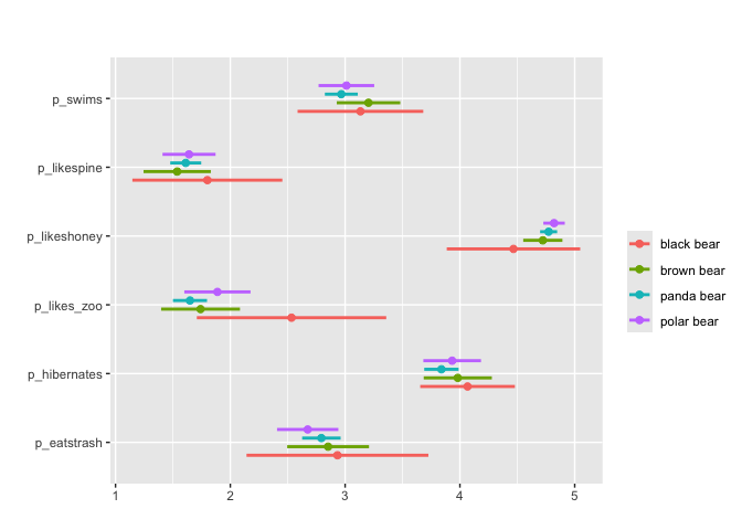

Finally, for Likert questions (scales of 3,5,7,9…) matrix_likert provides a custom plot

#you can specify custom labels with the `label` argument
matrix_likert(berlinbears,
              question = dplyr::starts_with('p_'),
              labels = c('Strongly disagree', 'Disagree','Neutral','Agree','Strongly agree'))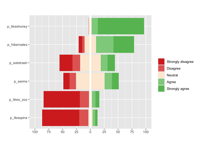

#can also apply pass custom colors and specify weights weights 
matrix_likert(berlinbears, 
              question = dplyr::starts_with('p_'),
              labels = c('Strongly disagree', 'Disagree','Neutral','Agree','Strongly agree'), 
              colors = c("#E1AA28", "#1E5F46", "#7E8F75", "#EFCD83", "#E17832"),
              weights = weights)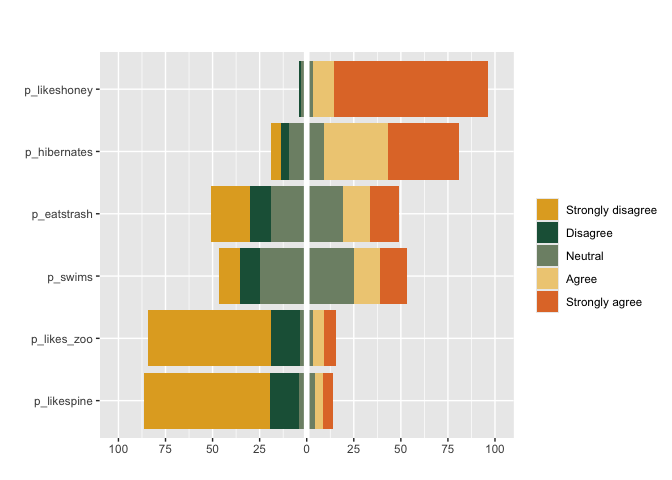 

Overview

Functions

• Single-choice
  • single_table
  • single_freq
• Multiple-choice
  • multi_table
  • multi_freq
• Matrix
  • matrix_table
  • matrix_freq
  • matrix_mean
  • matrix_likert

*_table functions return a gt table of the cross tabulations and frequencies for each question while *_freq returns the same data but as a plot.

For matrix-style questions with numerical input, matrix_mean plots the mean value value and ± two standard deviations. matrix_likert visualizes questions that accept Likert responses (strongly agree-strongly disagree) or questions with 3,5,7,9… categories.

Syntax

Each function contains the following options

• dataset —The input dataframe (or tibble) of survey questions
• question — The column(s) that contain the response options for a question, can be selected by using tidyselect semantics or providing a vector of column names or numbers
• group_by — Optional variable to group the analysis. If provided, the frequencies and counts will be calculated within each subgroup
• subgroups_to_exclude — Optional vector specifying subgroups to exclude from the analysis
• weights — Optional variable containing survey weights. If provided, frequencies and counts will be weighted accordingly
• na.rm — Logical indicating whether to remove NA values from question before analysis

These binaries (installable software) and packages are in development.
They may not be fully stable and should be used with caution. We make no claims about them.
Health stats visible at Monitor.