The hardware and bandwidth for this mirror is donated by dogado GmbH, the Webhosting and Full Service-Cloud Provider. Check out our Wordpress Tutorial.
If you wish to report a bug, or if you are interested in having us mirror your free-software or open-source project, please feel free to contact us at mirror[@]dogado.de.
The sshist package implements the Shimazaki-Shinomoto
method for finding the optimal number of bins in histograms.
Unlike the standard Freedman-Diaconis rule (used by default in ggplot2), this method minimizes the expected L2 loss function between the histogram and the unknown underlying density function. It is particularly effective for:
# stable version from CRAN
install.packages("sshist")
You can install the development version of sshist like so:
# install.packages("devtools")
devtools::install_github("celebithil/sshist")Here is a basic example using the Old Faithful Geyser data.
library(sshist)

# Load data
data(faithful)
x_data <- faithful$waiting

# Calculate optimal binning
res <- sshist(x_data)

# Print summary
print(res)
#> Shimazaki-Shinomoto Histogram Optimization
#> ------------------------------------------
#> Optimal Bins (N): 21
#> Bin Width (D):    2.524
#> Cost Minimum:     -8.525

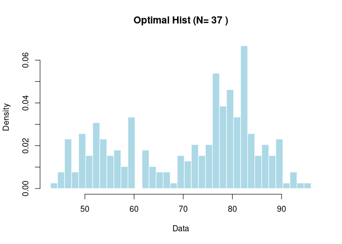
hist(res$data, breaks=res$edges, freq=FALSE,
       main=paste("Optimal Hist (N=", res$opt_n, ")"),
       col="lightblue", border="white", xlab="Data")
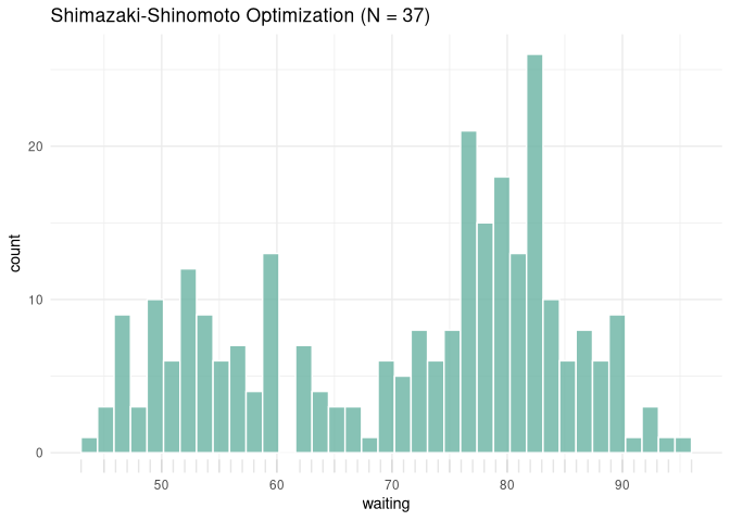
sshist calculates the optimal parameters, which you can
easily pass to ggplot2.
library(ggplot2)

# Create a data frame
df <- data.frame(waiting = x_data)

ggplot(df, aes(x = waiting)) +
  geom_histogram(breaks = res$edges, fill = "#69b3a2", color = "white", alpha = 0.8) +
  geom_rug(alpha = 0.1) +
  ggtitle(paste0("Shimazaki-Shinomoto Optimization (N = ", res$opt_n, ")")) +
  theme_minimal()
For bivariate data, sshist_2d finds the optimal binning
for both X and Y axes simultaneously.
# Get bimodal 2D data
y_data <- faithful$eruptions

# Optimize
res2d <- sshist_2d(x_data, y_data)

# Print summary
print(res2d)
#> Shimazaki-Shinomoto 2D Histogram Optimization
#> ---------------------------------------------
#> Optimal Bins X:   9
#> Optimal Bins Y:   20
#> Bin Width X:      5.889
#> Bin Width Y:      0.175
#> Cost Minimum: -5.717You can easily use the optimized bin counts from
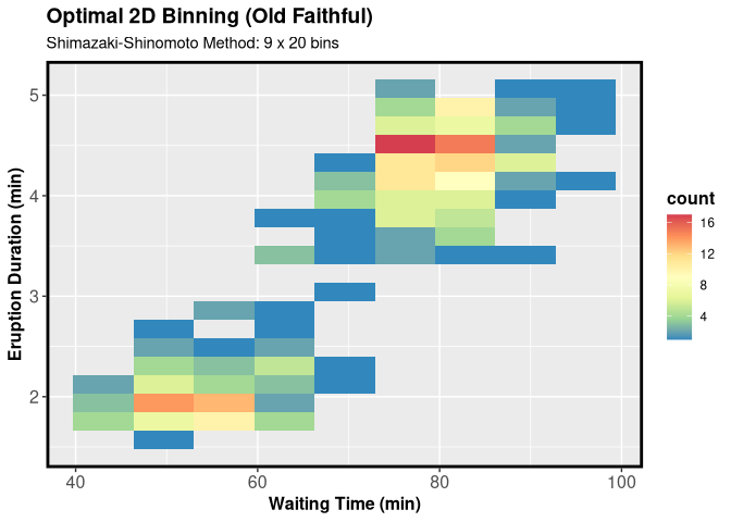
sshist_2d in ggplot2 by passing them to the
bins argument in geom_bin2d.
# We use the 'res2d' object calculated in Example 3
# containing optimal bins for Old Faithful data

res2d <- sshist_2d(faithful$waiting, faithful$eruptions )

ggplot(faithful, aes(waiting, eruptions)) +
  geom_bin2d(bins = c(res2d$opt_nx, res2d$opt_ny)) +
  scale_fill_distiller(palette = "Spectral") +
  labs(
    title = "Optimal 2D Binning (Old Faithful)",
    subtitle = paste0("Shimazaki-Shinomoto Method: ",
                      res2d$opt_nx, " x ", res2d$opt_ny, " bins"),
    x = "Waiting Time (min)",
    y = "Eruption Duration (min)"
  ) +
  theme(axis.text = element_text(size = 12),
        title = element_text(size = 12,face="bold"),
        panel.border = element_rect(linewidth = 2, color = "black", fill = NA))
These binaries (installable software) and packages are in development.
They may not be fully stable and should be used with caution. We make no claims about them.
Health stats visible at Monitor.