The hardware and bandwidth for this mirror is donated by dogado GmbH, the Webhosting and Full Service-Cloud Provider. Check out our Wordpress Tutorial.
If you wish to report a bug, or if you are interested in having us mirror your free-software or open-source project, please feel free to contact us at mirror[@]dogado.de.
![]()
![]()
Efficient superpixel segmentation for multi-band imagery using the
Simple Non-Iterative Clustering (SNIC) algorithm. The package wraps a
C++ implementation with an ergonomic R interface, integrates with
terra for raster workflows, and provides helpers for seed
placement, plotting, and reproducibility.
The snic package can be installed from CRAN:
install.packages("snic")Or the development version from GitHub:
# install.packages("remotes")
remotes::install_github("rolfsimoes/snic")
The terra package is suggested for raster support and
required for most of the plotting utilities demonstrated below.
arrays or
terra::SpatRaster objectssnic_grid(type = c("rectangular", "diamond", "hexagonal", "random"))
and interactive placement via snic_grid_manual()snic_plot()) for
quick inspection of inputs, seeds, and resulting segmentsterra (>= 1.7) is
suggested and is required for every raster example below. In-memory
array workflows can skip it, but you will lose the quick
plotting helpers.magick is optional
and only needed for snic_animation(). The chunk is cached
so missing the package merely skips the demo.SNIC produces compact superpixels in near-linear time and avoids the
iterative updates of SLIC-like algorithms. The snic package
exposes those speed benefits through:
terra integration, so you keep CRS, extent, and
metadata intact.The SNIC workflow is short and reproducible:
snic_grid() (rectangular,
diamond, hexagonal, or random layouts) or crafted interactively with
snic_grid_manual().snic() with
the chosen seeds to grow superpixels and inspect the result with
snic_plot() or the animated helper
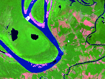
snic_animation().The example below demonstrates a typical SNIC workflow with the bundled Sentinel-2 subset.
library(snic)
library(terra)

# Sentinel-2 subset packaged with snic
data_dir <- system.file("demo-geotiff", package = "snic", mustWork = TRUE)
bands <- c("B02", "B04", "B08", "B12")
paths <- file.path(
  data_dir,
  sprintf("S2_20LMR_%s_20220630.tif", bands)
)
s2 <- terra::rast(paths)
names(s2) <- bands

# Visualise RGB composite with superpixel boundaries
snic_plot(
  s2,
  r = "B12", g = "B08", b = "B02",
  stretch = "lin"
)
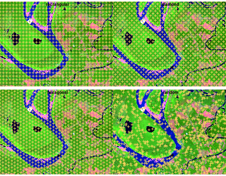
Seed placement controls the number, shape, and location of the
resulting superpixels. The package ships with several grid generators,
each returning a two-column (r, c) matrix
ready for snic():
snic_grid(type = "rectangular") - equally spaced seeds
along rows and columns.snic_grid(type = "diamond") - staggered rows produce a
diagonal pattern that better respects gradients.snic_grid(type = "hexagonal") - hexagonal tiling for
more isotropic superpixels.snic_grid(type = "random") - jittered seeds when
structure is irregular or prior knowledge is limited.Use snic_count_seeds() to forecast how many superpixels
a spacing will produce before running the algorithm.
set.seed(42)

grid_types <- c("rectangular", "diamond", "hexagonal", "random")
seed_examples <- lapply(grid_types, function(tp) {
    snic_grid(s2, type = tp, spacing = 30L, padding = 0L)
  }
)

op <- par(mfrow = c(2, 2), mar = c(1.5, 1.5, 2, 1))

for (i in seq_along(seed_examples)) {
  snic_plot(
    s2,
    r = 4, g = 3, b = 1,
    stretch = "lin",
    seeds = seed_examples[[i]],
    seeds_plot_args = list(pch = 3, col = "#F6D55C", lwd = 2)
  )
  title(grid_types[i])
}
snic_count_seeds(s2, spacing = 30L)
#> [1] 850

par(op)Automatic grids get you started quickly, but experts can refine seeds
interactively. snic_grid_manual() opens a plotting device
where you can add, move, or remove seeds on-the-fly and then feed the
result straight into snic():
manual_seeds <- snic_grid_manual(
  s2,
  base_seeds = seeds_rect,
  r = 4, g = 3, b = 1,
  stretch = "lin"
)

seg_manual <- snic(
  s2,
  seeds = manual_seeds,
  compactness = 0.1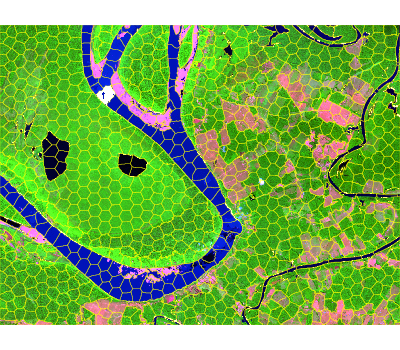
)Once seeds are defined, pass them to snic() together
with the imagery and a compactness factor. The result is a
labeled raster that can be visualized alongside the seeds for
validation.
seg_hex <- snic(s2, seeds = seed_examples[[3L]], compactness = 0.2)

snic_plot(
  s2,
  r = "B12", g = "B08", b = "B02",
  stretch = "lin",
  seg = seg_hex,
  seg_plot_args = list(border = "#FFFF00", col = NA, lwd = 0.6)
)
snic_animation() replays the seeding process, adding one
seed per frame, re-running snic(), and composing the frames
into a GIF. Cache the chunk so the animation is generated only once.
if (!requireNamespace("magick", quietly = TRUE)) {
  stop("Install the 'magick' package to render the animation.")
}

unlink("man/figures/segmentation-animation.gif")

set.seed(123)
animation_seeds <- snic_grid(s2, type = "random", spacing = 20L, padding = 0L)

gif_path <- snic_animation(
  s2,
  seeds = animation_seeds,
  file_path = "man/figures/segmentation-animation.gif",
  max_frames = 20L,
  delay = 30,
  r = 4, g = 3, b = 1,
  stretch = "lin",
  seeds_plot_args = list(pch = 16, col = "#00FFFF", cex = 1),
  seg_plot_args = list(border = "#FFD700", col = NA, lwd = 0.6),
  snic_args = list(compactness = 0.1),
  device_args = list(height = 192, width = 256, res = 120, bg = "white")
)
Bug reports, feature requests, and pull requests are welcome in the issue tracker. When proposing changes:
R CMD check or devtools::check() to
keep the package stable.README.Rmd if you touch code chunks so plots
stay in sync.terra,
magick) were available when reproducing a bug, as it
affects plotting and animation paths.These binaries (installable software) and packages are in development.
They may not be fully stable and should be used with caution. We make no claims about them.
Health stats visible at Monitor.