The hardware and bandwidth for this mirror is donated by dogado GmbH, the Webhosting and Full Service-Cloud Provider. Check out our Wordpress Tutorial.
If you wish to report a bug, or if you are interested in having us mirror your free-software or open-source project, please feel free to contact us at mirror[@]dogado.de.
![]()
![]()
simulariatools is an open source package with a collection of functions and tools useful to pre and post process data for air quality modelling and assessment:
contourPlot2() plots a production-ready contour map of
a pollutant concentration field.plotAvgRad() plots the hourly average of solar
radiation.plotAvgTemp() plots the average atmospheric
temperature.plotStabilityClass() plots histograms of atmospheric
stability class.vectorField() plots a simple vector field given two
components.importRaster() imports a generic raster file.importADSOBIN() imports an ADSO/BIN raster file.importSurferGrd() imports a grid file.stabilityClass() computes atmospheric stability
class.turnerStabilityClass() computes atmospheric PGT
stability class with Turner method.downloadBasemap() downloads GeoTIFF basemaps from the
Italian PCN.removeOutliers() removes time series outliers based on
interquartile range.rollingMax() computes rolling max of a time
series.The package is developed and maintained at Simularia and it is widely used in their daily work.
If you use this package in your work, please consider citing it. Refer to its Zenodo DOI to cite it.
To install the latest release of simulariatools from CRAN:
install.packages("simulariatools")NOTE: To import ADSO/BIN data files via
importADSOBIN(), a working installation of Python3 is required. For more information about R and Python interoperability, refer to the documentation ofreticulate.
To get bug fixes or to use a feature from the development version, install the development version from GitHub:
# install.packages("pak")
pak::pkg_install("Simularia/simulariatools")First, import air quality data from NetCDF or ADSO/BIN files with the appropriate convenience function:
library(simulariatools)
nox_concentration <- importRaster(
    file = "./development/conc_avg.nc",
    k = 1000,
    destaggering = TRUE,
    variable = "nox",
    verbose = TRUE
)
#> Raster statistics -----------------------------------------------
#>        X (min, max, dx)  :   496000.000   519250.000      250.000
#>        Y (min, max, dy)  :  4943000.000  4955250.000      250.000
#>      nox (min, max, mean):     0.00e+00     2.71e+00     1.52e-01
#> -----------------------------------------------------------------
Concentration data are imported as a data.frame with
x, y columns corresponding to the coordinates
of the cell centre and a z column for grid values.
str(nox_concentration)
#> 'data.frame':    4557 obs. of  3 variables:
#>  $ x: num  496125 496375 496625 496875 497125 ...
#>  $ y: num  4955125 4955125 4955125 4955125 4955125 ...
#>  $ z: num  0 0 0 0 0 0 0 0 0 0 ...
A quick contour plot, with default configuration, can be easily
obtained by running contourPlot2() without any
argument:
contourPlot2(nox_concentration)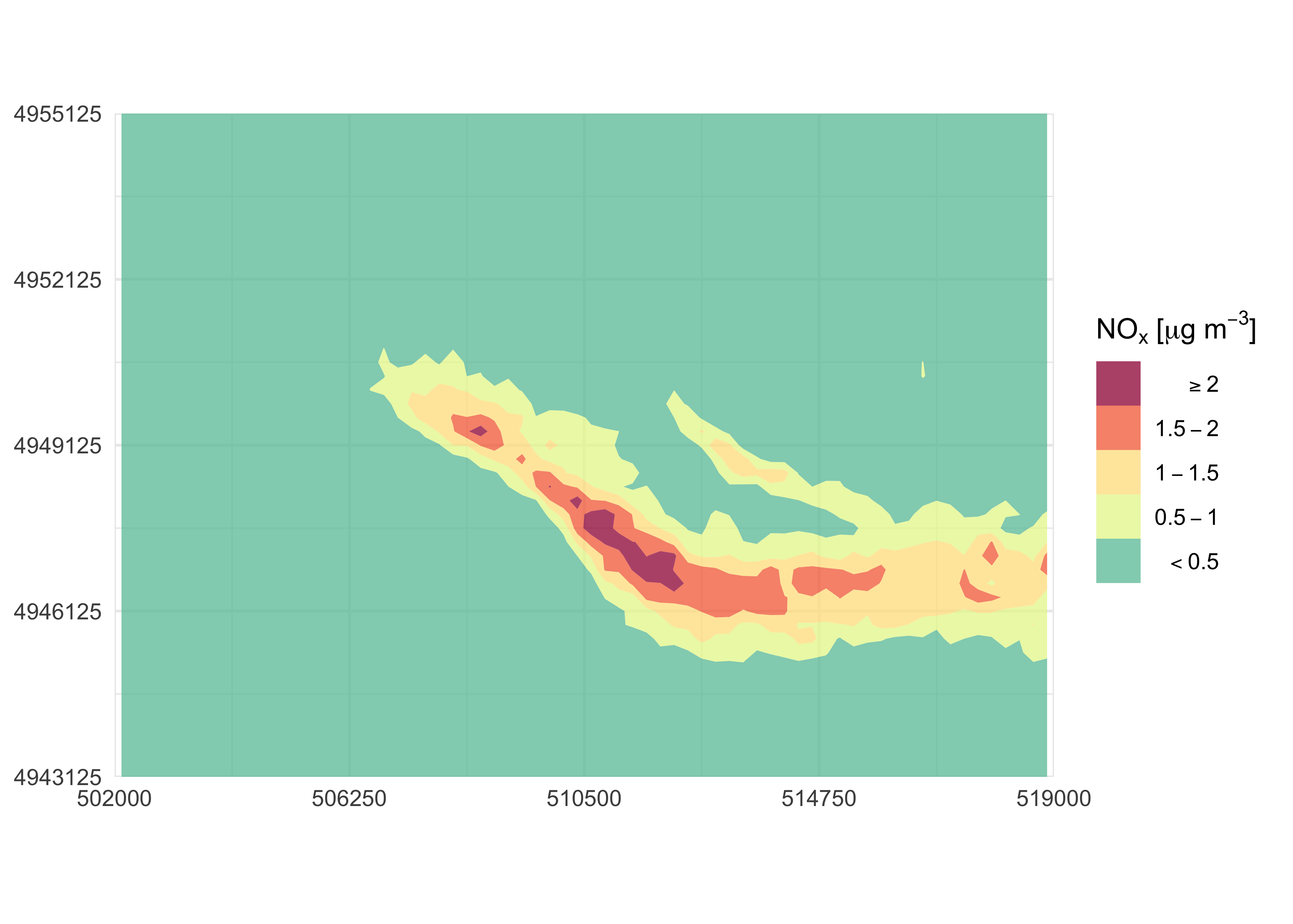
The plot is customisable by using contourPlot2()
arguments and by piping ggplot2 instructions together
with the + operator.
In the following example, the original domain is cropped, colour
levels are explicitly assigned and a legend name is provided through
function arguments. Furthermore, labs() and
theme_minimal() functions from ggplot2 are
used to remove axis labels and to change the overall theme:
library(ggplot2)
contourPlot2(
    nox_concentration,
    xlim = c(502000, 519000),
    ylim = c(4943125, 4955125),
    nticks = 5,
    levels = c(-Inf, 0.5, 1, 1.5, 2, Inf),
    legend = "NOx [ug/m3]"
) +
    labs(x = NULL, y = NULL) +
    theme_minimal()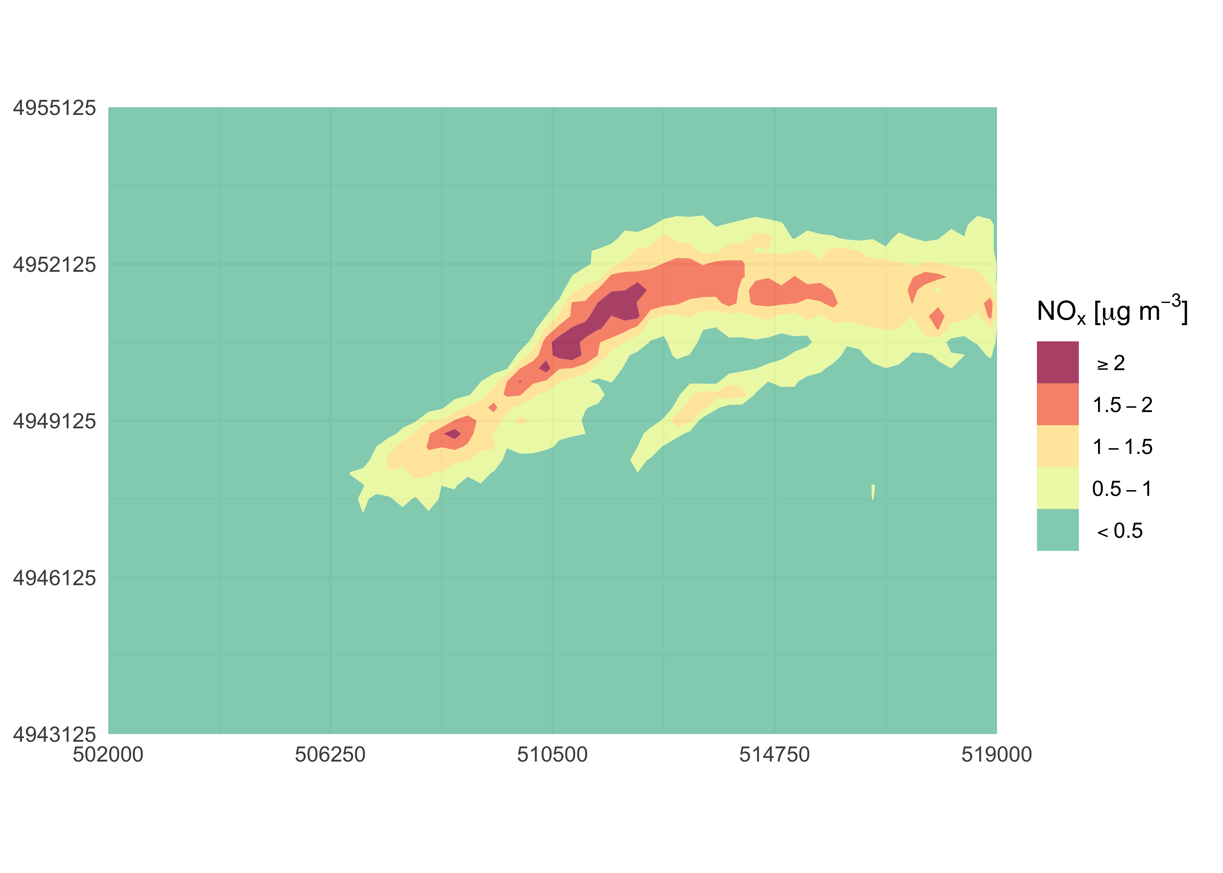
In order to save the last plot to file, you can directly use the
ggplot2 function ggsave():
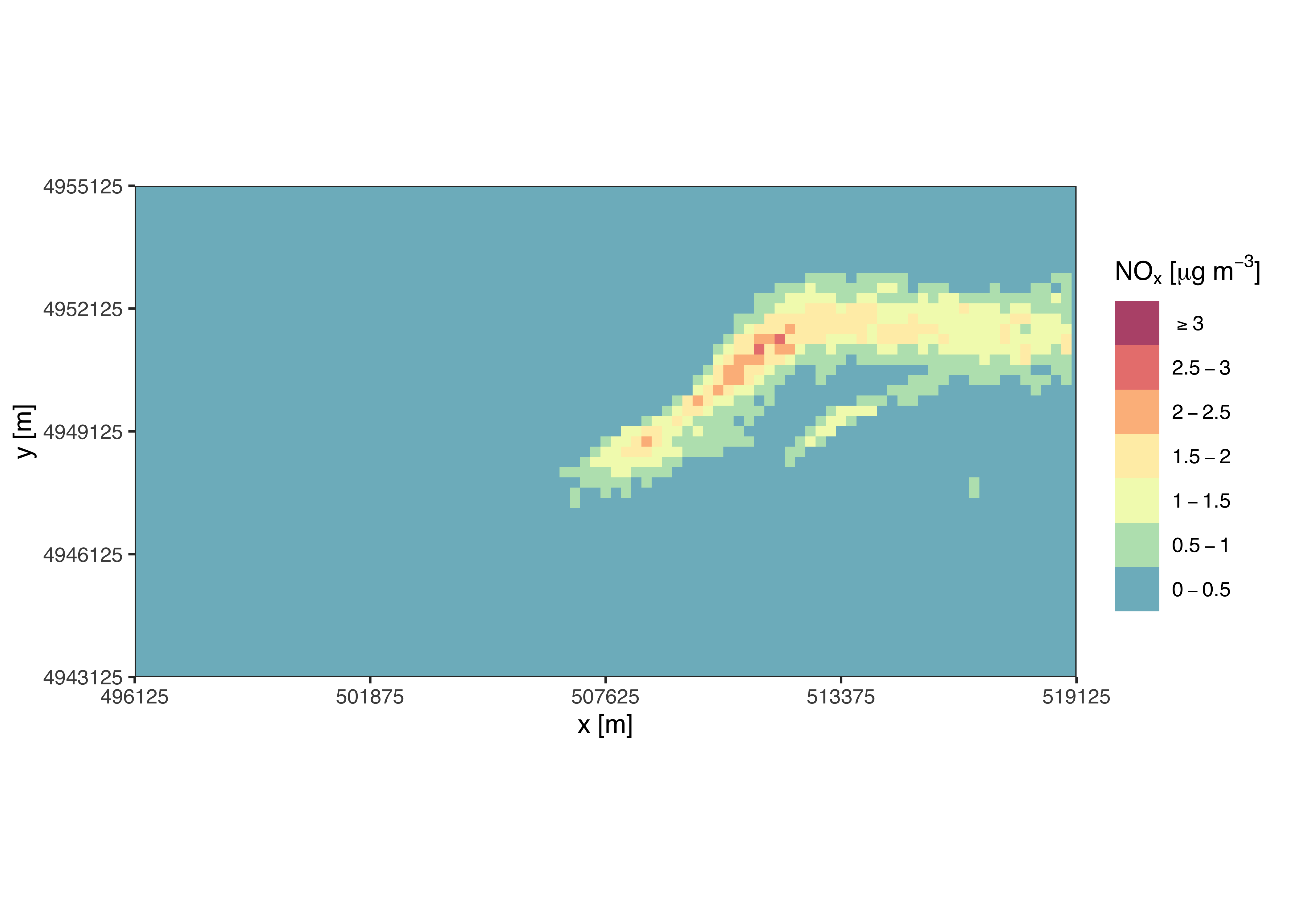
ggsave(filename = "~/path/to/myplot.png", width = 7, height = 6, dpi = 300)Optional arguments can be used to create special versions of the
plot. For example, use tile = TRUE to produce a
non-spatially interpolated plot:
contourPlot2(
    nox_concentration,
    tile = TRUE,
    legend = "NOx [ug/m3]"
)
Contact person:
Giuseppe Carlino (Simularia srl)
These binaries (installable software) and packages are in development.
They may not be fully stable and should be used with caution. We make no claims about them.
Health stats visible at Monitor.