simlandr:
Simulation-Based Landscape Construction for Dynamical Systems
The hardware and bandwidth for this mirror is donated by dogado GmbH, the Webhosting and Full Service-Cloud Provider. Check out our Wordpress Tutorial.
If you wish to report a bug, or if you are interested in having us mirror your free-software or open-source project, please feel free to contact us at mirror[@]dogado.de.
simlandr:
Simulation-Based Landscape Construction for Dynamical Systems
![]()
![]()
A toolbox for constructing potential landscapes for dynamical systems using Monte Carlo simulation. The method is based on the potential landscape definition by Wang et al. (2008) (also see Zhou & Li, 2016, for further mathematical discussions) and can be used for a large variety of models.
simlandr can help to:
hash_big_matrix class, and perform out-of-memory
calculation;You can install the released version of simlandr from CRAN with:
install.packages("simlandr")And you can install the development version from GitHub with:
install.packages("devtools")
devtools::install_github("Sciurus365/simlandr")
devtools::install_github("Sciurus365/simlandr", build_vignettes = TRUE) # Use this command if you want to build vignetteslibrary(simlandr)
# Simulation
## Single simulation
single_output_grad <- sim_fun_grad(length = 1e4, seed = 1614)
## Batch simulation: simulate a set of models with different parameter values
batch_arg_set_grad <- new_arg_set()
batch_arg_set_grad <- batch_arg_set_grad %>%
add_arg_ele(
arg_name = "parameter", ele_name = "a",
start = -6, end = -1, by = 1
)
batch_grid_grad <- make_arg_grid(batch_arg_set_grad)
batch_output_grad <- batch_simulation(batch_grid_grad, sim_fun_grad,
default_list = list(
initial = list(x = 0, y = 0),
parameter = list(a = -4, b = 0, c = 0, sigmasq = 1)
),
length = 1e4,
seed = 1614,
bigmemory = FALSE
)
batch_output_grad
#> Output(s) from 6 simulations.# Construct landscapes
## Example 1. 2D (x, y as U) landscape
l_single_grad_2d <- make_2d_static(single_output_grad, x = "x")
autoplot(l_single_grad_2d)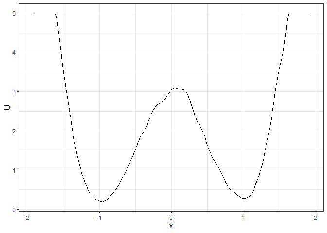
### To make the landscape smoother
make_2d_static(single_output_grad, x = "x", adjust = 5) %>% autoplot()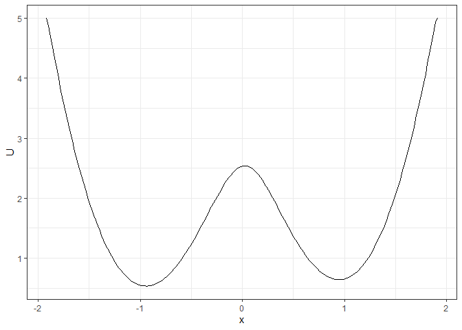
## Example 2. 3D (x, y, color as U) landscape
l_single_grad_3d <- make_3d_static(single_output_grad, x = "x", y = "y", adjust = 5)
autoplot(l_single_grad_3d)
### plotly_ld(l_single_grad_3d) # to show the landscape in 3D (x, y, z)

## Example 3. 4D (x, y, z, color as U) landscape
set.seed(1614)
single_output_grad <- matrix(runif(nrow(single_output_grad), min = 0, max = 5), ncol = 1, dimnames = list(NULL, "z")) %>% cbind(single_output_grad)
l_single_grad_4d <- make_4d_static(single_output_grad, x = "x", y = "y", z = "z", n = 50)
### plotly_ld(l_single_grad_4d) # to show the landscape in 4D (x, y, z, color as U)

## Example 4. 2D (x, y as U) matrix (by a)
l_batch_grad_2d <- make_2d_matrix(batch_output_grad, x = "x", cols = "a", Umax = 8, adjust = 2)
autoplot(l_batch_grad_2d)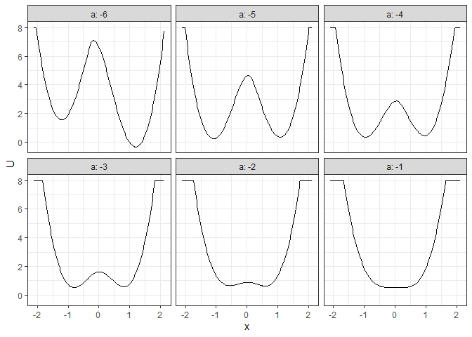
## Example 5. 3D (x, y, color as U) matrix (by a)
l_batch_grad_3d <- make_3d_matrix(batch_output_grad, x = "x", y = "y", cols = "a")
autoplot(l_batch_grad_3d)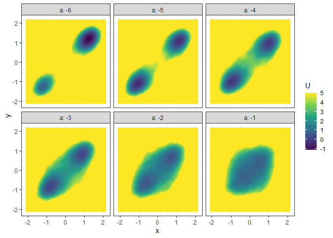
## Example 6. 3D (x, y, z/color as U) animation (by a)
l_batch_grad_3d_animation <- make_3d_animation(batch_output_grad, x = "x", y = "y", fr = "a")
### plotly_ld(l_batch_grad_3d_animation) # landscape animation in 3D (x, y, z as U)
### autoplot(l_batch_grad_3d_animation) # animation with color as U
# Calculate energy barriers
## Example 1. Energy barrier for the 2D landscape
b_single_grad_2d <- calculate_barrier(l_single_grad_2d,
start_location_value = -1, end_location_value = 1,
start_r = 0.3, end_r = 0.3
)
summary(b_single_grad_2d)
#> delta_U_start delta_U_end
#> 2.896270 2.806378
autoplot(l_single_grad_2d) + autolayer(b_single_grad_2d)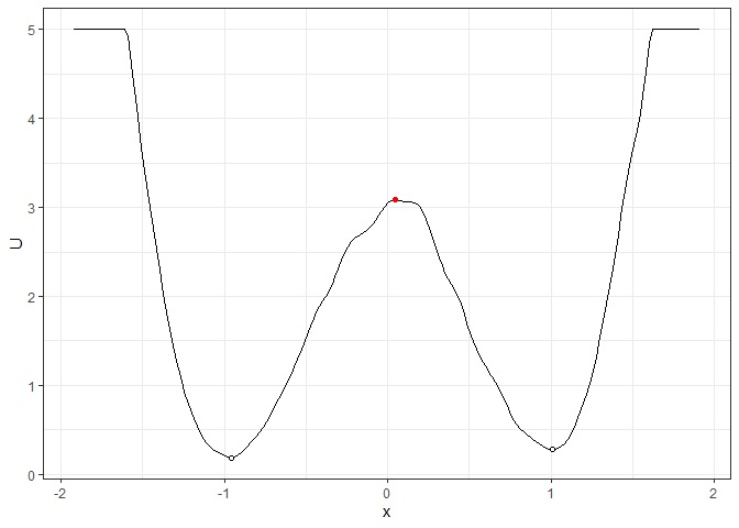
## Example 2. Energy barrier for the 3D landscape
b_single_grad_3d <- calculate_barrier(l_single_grad_3d,
  start_location_value = c(-1, -1), end_location_value = c(1, 1),
  start_r = 0.3, end_r = 0.3
)
summary(b_single_grad_3d)
#> delta_U_start   delta_U_end
#>      3.491516      3.360399
autoplot(l_single_grad_3d) + autolayer(b_single_grad_3d)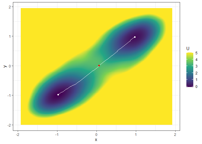
## Example 3. Energy barrier for many 2D landscapes
b_batch_grad_2d <- calculate_barrier(l_batch_grad_2d,
  start_location_value = -1, end_location_value = 1,
  start_r = 0.3, end_r = 0.3
)
summary(b_batch_grad_2d)
#> # A tibble: 6 × 9
#>   start_x start_U end_x  end_U saddle_x saddle_U  cols delta_U_start delta_U_end
#>     <dbl>   <dbl> <dbl>  <dbl>    <dbl>    <dbl> <dbl>         <dbl>       <dbl>
#> 1  -1.21    1.56  1.21  -0.332  -0.171     7.10     -6         5.54       7.43
#> 2  -1.08    0.243 1.08   0.348   0.0418    4.65     -5         4.40       4.30
#> 3  -0.957   0.355 0.977  0.454   0.0418    2.87     -4         2.52       2.42
#> 4  -0.808   0.530 0.807  0.572   0.0205    1.62     -3         1.09       1.05
#> 5  -0.702   0.710 0.700  0.659   0.0205    0.884    -2         0.174      0.225
#> 6  -0.702   0.895 0.700  0.834  -0.702     0.895    -1         0          0.0613
autoplot(l_batch_grad_2d) + autolayer(b_batch_grad_2d)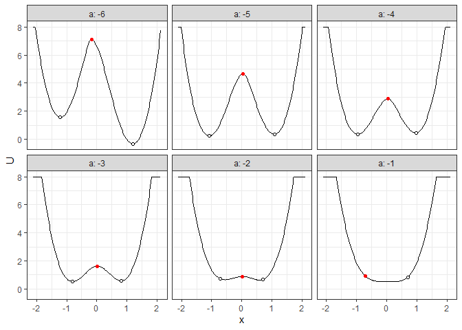
## Example 4. Energy barrier for many 3D landscapes
b_batch_grad_3d <- calculate_barrier(l_batch_grad_3d,
  start_location_value = c(-1, -1), end_location_value = c(1, 1),
  start_r = 0.3, end_r = 0.3
)
summary(b_batch_grad_3d)
#> # A tibble: 6 × 12
#>   start_x start_y start_U end_x end_y  end_U  saddle_x  saddle_y saddle_U  cols
#>     <dbl>   <dbl>   <dbl> <dbl> <dbl>  <dbl>     <dbl>     <dbl>    <dbl> <dbl>
#> 1  -1.21   -1.21   0.735  1.21  1.21  -1.14  -0.213    -0.259        9.40    -6
#> 2  -1.08   -1.10  -0.480  1.10  1.12  -0.369  0.0843    0.151        5.40    -5
#> 3  -0.978  -0.992 -0.257  0.977 0.993 -0.133  0.0843    0.000337     3.60    -4
#> 4  -0.851  -0.820  0.0797 0.849 0.820  0.148  0.0843    0.108        1.99    -3
#> 5  -0.702  -0.712  0.608  0.700 0.712  0.466 -0.000710  0.0866       1.33    -2
#> 6  -0.702  -0.712  1.12   0.700 0.712  1.11  -0.702    -0.712        1.12    -1
#> # … with 2 more variables: delta_U_start <dbl>, delta_U_end <dbl>
autoplot(l_batch_grad_3d) + autolayer(b_batch_grad_3d)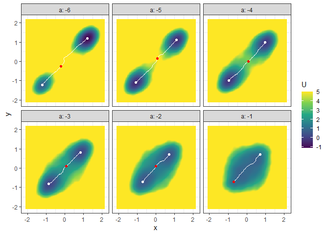
See the vignettes of this package
(browseVignettes("simlandr") or https://doi.org/10.31234/osf.io/pzva3) for more examples
and explanations. Also see https://doi.org/10.1080/00273171.2022.2119927 for our
recent work using simlandr.
These binaries (installable software) and packages are in development.
They may not be fully stable and should be used with caution. We make no claims about them.
Health stats visible at Monitor.