The hardware and bandwidth for this mirror is donated by dogado GmbH, the Webhosting and Full Service-Cloud Provider. Check out our Wordpress Tutorial.
If you wish to report a bug, or if you are interested in having us mirror your free-software or open-source project, please feel free to contact us at mirror[@]dogado.de.
results <- dist_search(x, y, max_distance = 2, nthreads = 1)The above code will find all similar sequences/strings between
x and y. This will generally be significantly
faster than calculating pairwise distance or pairwise alignment.
seqtrie is a collection of Radix Tree algorithms. These
include some classic algorithms like prefix lookup and more
bioinformatics focused algorithms such as alignment algorithms and
sequence distance calculations (Hamming and Levenshtein distances).
A trie (aka Prefix Tree) is a data structure used in many applications. It is a space efficient data structure where a collection of sequences are stored in a tree structure, where each leaf represents one sequence, and each node holds one character representing a shared prefix of all sequences descending from it. A Radix Tree (aka Compact Prefix Tree) is an improvement on a trie, using less memory and being generally faster. In a Radix Tree, each node is able to represent multiple characters instead of just one.
Tries and Radix Trees have similar complexity to a hashmap. Storing a sequence within the tree or looking it up are O(k) where k is the length of the sequence. The main advantage of a trie is that it can be used to quickly find similar sequences by various algorithms and metrics, whereas a hashmap does not contain any sequence similarity information.
See also: https://en.wikipedia.org/wiki/Radix_tree
In seqtrie, there are two R6 classes:
RadixTree is the primary class in this package. There
are three main methods. The $insert() method is used to
store sequences on the tree, $erase() for erasing sequences
from the tree and $search() for finding similar sequences
stored on the tree.
The second R6 class is RadixForest, a
derivative data structure where separate trees are constructed for each
sequence length. This data structure has advantages and disadvantages,
discussed later.
Finally, there’s a simple convenience function
dist_search to find similar sequences using a
RadixTree or RadixForest object. This is a
wrapper around the $new, $insert and
$search() methods.
install.packages("seqtrie")
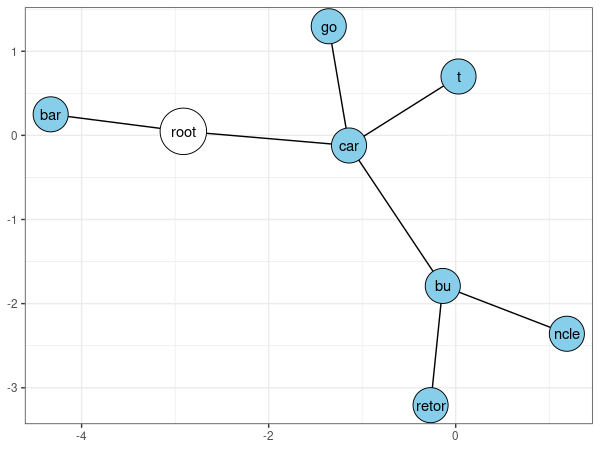
Below is a simple example where we insert some sequences (strings), erase one and then plot out the tree.
tree <- RadixTree$new()
tree$insert(c("cargo", "cart", "carburetor", "carbuncle", "bar", "zebra"))
tree$erase("zebra")
# tree$graph requires igraph package
set.seed(1); tree$graph()
Below is an example using COVID19 T-cell data from Adaptive Biotechnologies. (doi: 10.21203/rs.3.rs-51964/v1. This data is licensed under CC 4.0.)
Here, we find highly similar sequences within a fixed edit distance. For the purpose of this vignette, we sample a small selection of sequences.
On the full dataset, if you tried to calculate an edit distance matrix, it would take a pretty long time, not to mention requiring a lot of memory. A trie-based method could be used to find similar sequences in a fraction of the time. Approximate running times on the full dataset using 8 threads are listed in the comments.
# 130,000 "CDR3" sequences
set.seed(1)
data(covid_cdr3)
covid_cdr3 <- sample(covid_cdr3, 1000)
tree <- RadixTree$new()
tree$insert(covid_cdr3)
# Full data: 1 min
results <- tree$search(covid_cdr3, max_distance=2, mode="levenshtein", nthreads=2)

# Alternatively, instead of using the RadixTree object directly, you can use the
# dist_search function, which is a wrapper around the RadixTree object.
results <- dist_search(covid_cdr3, covid_cdr3, max_distance=2)

# The output is a data.frame mapping query (search sequences)
# and target (sequences inserted into the tree).
dplyr::filter(results, query != target)
## query
## 1 TGTGCCAGCAGTCACGGAACTAGCACAGATACGCAGTATTTT
## 2 TGCAGCGTTGATCTGCCGGGAGAGACCCAGTACTTC
## 3 TGTGCCAGTACTATGGGACAGGGGATGAACACTGAAGCTTTCTTT
## 4 TGTGCCAGTAGTATGGGACAGGGAATGAACACTGAAGCTTTCTTT
## 5 TGTGCCAGCAGTGACAGAACTAGCACAGATACGCAGTATTTT
## 6 TGCAGCGTTGATCTGACGGGAGAGACCCAGTACTTC
## target distance
## 1 TGTGCCAGCAGTGACAGAACTAGCACAGATACGCAGTATTTT 2
## 2 TGCAGCGTTGATCTGACGGGAGAGACCCAGTACTTC 1
## 3 TGTGCCAGTAGTATGGGACAGGGAATGAACACTGAAGCTTTCTTT 2
## 4 TGTGCCAGTACTATGGGACAGGGGATGAACACTGAAGCTTTCTTT 2
## 5 TGTGCCAGCAGTCACGGAACTAGCACAGATACGCAGTATTTT 2
## 6 TGCAGCGTTGATCTGCCGGGAGAGACCCAGTACTTC 1The $search() function contains two mutually exclusive
parameters: max_distance and max_fraction.The
former parameter sets an absolute threshold that limits the distance
between pairs of sequences in the output, and the latter parameter sets
a threshold relative to the query sequence length.
The search time is monotonically increasing with the distance threshold, logarithmically increasing with tree size and linearly increasing with the number of query sequences and the length of each sequence. Overall, the algorithm is significantly faster than a pairwise/matrix edit distance calculation for finding similar sequences. However, care still needs to be taken when setting parameters for searching a large number of sequences (~100,000+).
Some additional examples using the max_fraction parameter.
# Full data: several seconds
results <- tree$search(covid_cdr3, max_fraction=0.035, mode="levenshtein", nthreads=2)
# Full data: 1 minute
results <- tree$search(covid_cdr3, max_fraction=0.06, mode="levenshtein", nthreads=2)
# Full data: 15-20 minutes
results <- tree$search(covid_cdr3, max_fraction=0.15, mode="levenshtein", nthreads=2)
Hamming distance is similar to Levenshtein distance, but does not allow insertions or deletions. Sequences must be the same length. Because of this restriction, Hamming distance is generally a lot faster.
# Full data: 1 second
results <- tree$search(covid_cdr3, max_fraction=0.035, mode="hamming", nthreads=2)
# Full data: several seconds
results <- tree$search(covid_cdr3, max_fraction=0.06, mode="hamming", nthreads=2)
# Full data: 1.5 minutes
results <- tree$search(covid_cdr3, max_fraction=0.15, mode="hamming", nthreads=2)An anchored alignment is a form of semi-global alignment, where the query sequence is “anchored” (global) to the beginning of both the query and target sequences, but is semi-global in that the end of the either the query sequence or target sequence (but not both) can be unaligned. This type of alignment is sometimes called an “extension” alignment in literature.
tree <- RadixTree$new()
tree$insert("CARTON")
tree$insert("CAR")
tree$insert("CARBON")
tree$search("CART", max_distance = 0, mode = "anchored")
## query target distance query_size target_size
## 1 CART CAR 0 3 3
## 2 CART CARTON 0 4 4Because the alignment is semi-global at the end of the alignment, the query of “CART” finds “CAR” and “CARTON” but not “CARBON” given a max distance of 0. Additionally, the output of an anchored search also returns the position of the query and target at the ends. Either the query or the target must fully align, so at least one of the end positions will be the full length of the sequence. This type of alignment is frequently useful in biology e.g. if you are trying to align multiple reads that are variable in length but start at the same genomic position or primer site.
seqtrie supports custom substitution costs and affine
gap penalties. Note: we are calculating distance (higher is worse) and
not alignment score (higher is better).
tree <- RadixTree$new()
tree$insert(covid_cdr3)

# Define a custom substitution matrix. Use generate_cost_matrix for convenience.
cost_mat <- generate_cost_matrix("ACGT", match = 0, mismatch = 5)
print(cost_mat)
## A C G T
## A 0 5 5 5
## C 5 0 5 5
## G 5 5 0 5
## T 5 5 5 0# Set gap penalties via parameters (not in the matrix):
# - Linear gaps: set gap_cost only
# - Affine gaps: set both gap_cost and gap_open_cost
# Linear example
results_linear <- tree$search(covid_cdr3, max_distance = 8,
mode = "global",
cost_matrix = cost_mat,
gap_cost = 2,
nthreads = 2)
# Affine example
results_affine <- tree$search(covid_cdr3, max_distance = 8,
mode = "global",
cost_matrix = cost_mat,
gap_cost = 2,
gap_open_cost = 5,
nthreads = 2)
dplyr::filter(results_linear, query != target)## query
## 1 TGTGCCAGCAGCTTAGGACAGTCCTACGAGCAGTACTTC
## 2 TGTGCCAGCAGCTTAGGACAGTCCTACGAGCAGTACTTC
## 3 TGTGCCAGCAGTCACGGAACTAGCACAGATACGCAGTATTTT
## 4 TGCAGCGTTGATCTGCCGGGAGAGACCCAGTACTTC
## 5 TGTGCCAGCAGCTCGGCGGGGTCCTACAATGAGCAGTTCTTC
## 6 TGTGCCAGCAGTTACGGGCAGTCCTACGAGCAGTACTTC
## 7 TGTGCCAGCAGTTACGGGCAGTCCTACGAGCAGTACTTC
## 8 TGTGCCAGTACTATGGGACAGGGGATGAACACTGAAGCTTTCTTT
## 9 TGTGCCAGTAGTATGGGACAGGGAATGAACACTGAAGCTTTCTTT
## 10 TGTGCCAGCAGCTCAGGGGGCTCCTACAATGAGCAGTTCTTC
## 11 TGTGCCAGCAGTTGGGGGGGCTACGAGCAGTACTTC
## 12 TGTGCCAGCAGTTCCCCTAATAGCAATCAGCCCCAGCATTTT
## 13 TGTGCCAGCAGTTTATCGGGGTCCTACGAGCAGTACTTC
## 14 TGTGCCAGCAGTTTATCGGGGTCCTACGAGCAGTACTTC
## 15 TGTGCCAGCAGCCTTAGCGGGGTGAGCACAGATACGCAGTATTTT
## 16 TGTGCCAGCAGTCCCTCAGGGGAGACCCAGTACTTC
## 17 TGTGCCAGCAGCCTAGCAGGGGCCGGGGAGCTGTTTTTT
## 18 TGTGCCAGCAGGCCAGGACAGTCCTACGAGCAGTACTTC
## 19 TGTGCCAGCAGCTTAGAGGCGGCCGGGGAGCTGTTTTTT
## 20 TGTGCCAGCAGTCCCATAGATAGCAATCAGCCCCAGCATTTT
## 21 TGTGCCAGCAGTGACAGAACTAGCACAGATACGCAGTATTTT
## 22 TGTGCCAGCAGTTTAGGGGGTGGCTACGAGCAGTACTTC
## 23 TGTGCCAGCAGTTTCGGGGCCTACGAGCAGTACTTC
## 24 TGTGCCAGCAGCCTTAGCGGTAGCACAGATACGCAGTATTTT
## 25 TGTGCCAGCAGTCCTAGCGGCGAGACCCAGTACTTC
## 26 TGCAGCGTTGATCTGACGGGAGAGACCCAGTACTTC
## target distance
## 1 TGTGCCAGCAGTTACGGGCAGTCCTACGAGCAGTACTTC 8
## 2 TGTGCCAGCAGGCCAGGACAGTCCTACGAGCAGTACTTC 8
## 3 TGTGCCAGCAGTGACAGAACTAGCACAGATACGCAGTATTTT 8
## 4 TGCAGCGTTGATCTGACGGGAGAGACCCAGTACTTC 4
## 5 TGTGCCAGCAGCTCAGGGGGCTCCTACAATGAGCAGTTCTTC 8
## 6 TGTGCCAGCAGTTTATCGGGGTCCTACGAGCAGTACTTC 8
## 7 TGTGCCAGCAGCTTAGGACAGTCCTACGAGCAGTACTTC 8
## 8 TGTGCCAGTAGTATGGGACAGGGAATGAACACTGAAGCTTTCTTT 8
## 9 TGTGCCAGTACTATGGGACAGGGGATGAACACTGAAGCTTTCTTT 8
## 10 TGTGCCAGCAGCTCGGCGGGGTCCTACAATGAGCAGTTCTTC 8
## 11 TGTGCCAGCAGTTTAGGGGGTGGCTACGAGCAGTACTTC 6
## 12 TGTGCCAGCAGTCCCATAGATAGCAATCAGCCCCAGCATTTT 8
## 13 TGTGCCAGCAGTTTCGGGGCCTACGAGCAGTACTTC 6
## 14 TGTGCCAGCAGTTACGGGCAGTCCTACGAGCAGTACTTC 8
## 15 TGTGCCAGCAGCCTTAGCGGTAGCACAGATACGCAGTATTTT 6
## 16 TGTGCCAGCAGTCCTAGCGGCGAGACCCAGTACTTC 8
## 17 TGTGCCAGCAGCTTAGAGGCGGCCGGGGAGCTGTTTTTT 8
## 18 TGTGCCAGCAGCTTAGGACAGTCCTACGAGCAGTACTTC 8
## 19 TGTGCCAGCAGCCTAGCAGGGGCCGGGGAGCTGTTTTTT 8
## 20 TGTGCCAGCAGTTCCCCTAATAGCAATCAGCCCCAGCATTTT 8
## 21 TGTGCCAGCAGTCACGGAACTAGCACAGATACGCAGTATTTT 8
## 22 TGTGCCAGCAGTTGGGGGGGCTACGAGCAGTACTTC 6
## 23 TGTGCCAGCAGTTTATCGGGGTCCTACGAGCAGTACTTC 6
## 24 TGTGCCAGCAGCCTTAGCGGGGTGAGCACAGATACGCAGTATTTT 6
## 25 TGTGCCAGCAGTCCCTCAGGGGAGACCCAGTACTTC 8
## 26 TGCAGCGTTGATCTGCCGGGAGAGACCCAGTACTTC 4The RadixForest class is a data structure holding a
collection of Radix Trees, where a separate tree is constructed for each
sequence length. The primary advantage of RadixForest is
significantly faster Levenshtein searches, because you can know sequence
length up front. The disadvantages are higher memory usage, and no
support for custom distance searches.
Below is a brief comparison:
# RadixTree, full data: 45 seconds
tree <- RadixTree$new()
tree$insert(covid_cdr3)
results_tree <- tree$search(covid_cdr3, max_distance=2, mode="levenshtein", nthreads=2)
# RadixForest, full data: 19 seconds
frst <- RadixForest$new()
frst$insert(covid_cdr3)
results_frst <- frst$search(covid_cdr3, max_distance=2, mode="levenshtein", nthreads=2)
# The results are the same, but order is not guaranteed
identical(
  dplyr::arrange(results_tree, query, target),
  dplyr::arrange(results_frst, query, target) )
## [1] TRUEThe $prefix_search() function can be used to find
similar sequences that start with a pattern. This is one of the classic
use cases of trie data structures, for use as a database lookup and
predictive text.
tree <- RadixTree$new()
tree$insert(c("cargo", "cart", "carburetor", "carbuncle", "bar"))
tree$prefix_search("car")
## query target
## 1 car cargo
## 2 car cart
## 3 car carburetor
## 4 car carbuncleThese binaries (installable software) and packages are in development.
They may not be fully stable and should be used with caution. We make no claims about them.
Health stats visible at Monitor.