The hardware and bandwidth for this mirror is donated by dogado GmbH, the Webhosting and Full Service-Cloud Provider. Check out our Wordpress Tutorial.
If you wish to report a bug, or if you are interested in having us mirror your free-software or open-source project, please feel free to contact us at mirror[@]dogado.de.

saens

Author

Ridson Al Farizal P, Azka Ubaidillah

Maintainer

Ridson Al Farizal P ridsonap@bps.go.id

Description

EBLUP Fay-Herriot Model for Estimation of Non-Sampled Areas with Cluster Information.

Installation

You can install the development version of saens from GitHub with:

# install.packages("devtools")
devtools::install_github("Alfrzlp/saens")

or you can install cran version

install.packages("saens")

Example

This is a basic example which shows you how to solve a common problem:

library(saens)
library(dplyr)
library(tidyr)
library(ggplot2)

windowsFonts(
  poppins = windowsFont('poppins')
)

Data

milk$var <- milk$SD^2

# glimpse(mys)
# glimpse(milk)

EBLUP Model

model1 <- eblupfh(yi ~ as.factor(MajorArea), data = milk, vardir = "var")
#> ✔ Convergence after 4 iterations
#> → Method : REML
#> 
#> ── Coefficient ─────────────────────────────────────────────────────────────────
#>                            beta Std.Error z-value   p-value    
#> (Intercept)            0.968189  0.069362 13.9585 < 2.2e-16 ***
#> as.factor(MajorArea)2  0.132780  0.103001  1.2891  0.197357    
#> as.factor(MajorArea)3  0.226946  0.092330  2.4580  0.013972 *  
#> as.factor(MajorArea)4 -0.241301  0.081617 -2.9565  0.003111 ** 
#> ---
#> Signif. codes:  0 '***' 0.001 '**' 0.01 '*' 0.05 '.' 0.1 ' ' 1

AIC, BIC, and Loglikehood

AIC(model1)
#>       AIC 
#> -15.35496
BIC(model1)
#>       BIC 
#> -6.548956
logLik(model1)
#>  loglike 
#> 12.67748

Coef

coef(model1)
#>           (Intercept) as.factor(MajorArea)2 as.factor(MajorArea)3 
#>             0.9681890             0.1327801             0.2269462 
#> as.factor(MajorArea)4 
#>            -0.2413011

Summary

summary(model1)
#>                            beta Std.Error z-value   p-value    
#> (Intercept)            0.968189  0.069362 13.9585 < 2.2e-16 ***
#> as.factor(MajorArea)2  0.132780  0.103001  1.2891  0.197357    
#> as.factor(MajorArea)3  0.226946  0.092330  2.4580  0.013972 *  
#> as.factor(MajorArea)4 -0.241301  0.081617 -2.9565  0.003111 ** 
#> ---
#> Signif. codes:  0 '***' 0.001 '**' 0.01 '*' 0.05 '.' 0.1 ' ' 1

Autoplot

saens::autoplot(model1, variable = 'MSE')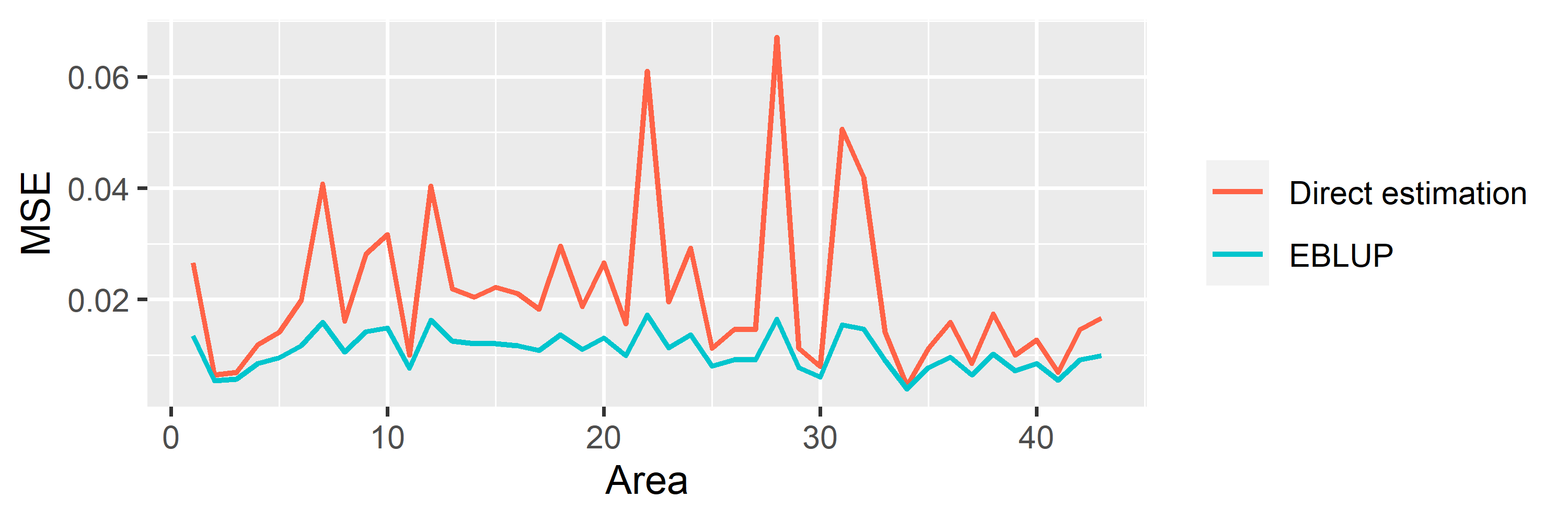

saens::autoplot(model1, variable = 'RRMSE')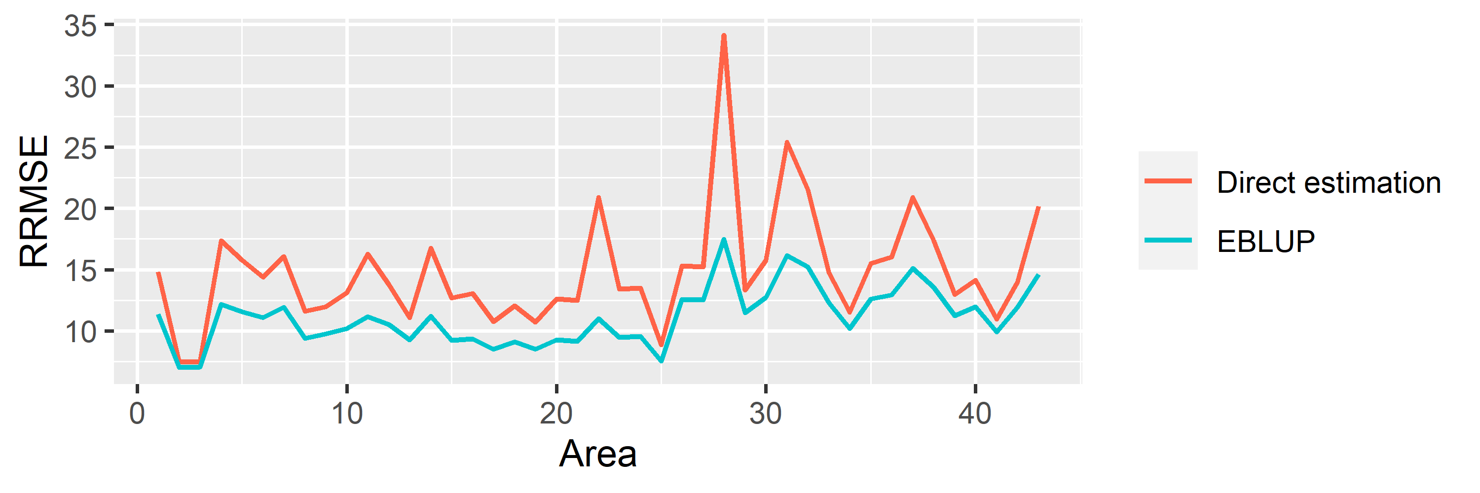

saens::autoplot(model1, variable = 'estimation')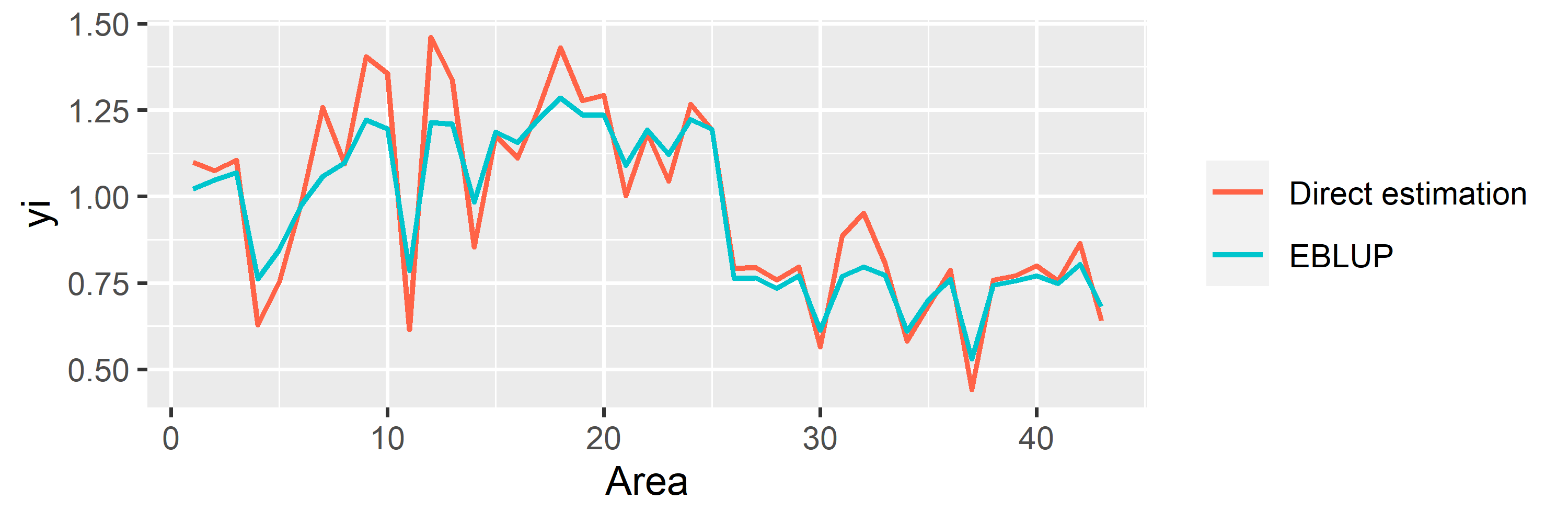

EBLUP Model for Non-sampled Areas

model_ns <- eblupfh_cluster(y ~ x1 + x2 + x3, data = mys, vardir = "var", cluster = "clust")
#> ✔ Convergence after 6 iterations
#> → Method : REML
#> 
#> ── Coefficient ─────────────────────────────────────────────────────────────────
#>                   beta  Std.Error z-value   p-value    
#> (Intercept)  3.1077510  0.7697687  4.0373 5.408e-05 ***
#> x1          -0.0019323  0.0098886 -0.1954    0.8451    
#> x2           0.0555184  0.0614129  0.9040    0.3660    
#> x3           0.0335344  0.0580013  0.5782    0.5632    
#> ---
#> Signif. codes:  0 '***' 0.001 '**' 0.01 '*' 0.05 '.' 0.1 ' ' 1

Comparison of estimates and RSE

mys$eblup_est <- model_ns$df_res$eblup
mys$eblup_rse <- model_ns$df_res$rse
  
glimpse(mys)
#> Rows: 42
#> Columns: 10
#> $ area      <int> 1, 2, 3, 4, 5, 6, 7, 8, 9, 10, 11, 12, 13, 14, 15, 16, 17, 1…
#> $ y         <dbl> 8.359527, 7.599650, 5.514137, 3.869326, 6.305063, 3.926807, …
#> $ var       <dbl> 0.6618838, 0.8374691, 0.8822257, 0.6581716, 1.2788021, 0.387…
#> $ rse       <dbl> 9.732158, 12.041783, 17.033831, 20.966899, 17.935449, 15.858…
#> $ x1        <dbl> 124, 89, 57, 88, 141, 96, 146, 110, 58, 63, 35, 56, 84, 240,…
#> $ x2        <dbl> 24, 18, 19, 35, 46, 29, 57, 41, 18, 13, 12, 14, 38, 71, 33, …
#> $ x3        <dbl> 14, 9, 5, 19, 29, 10, 34, 23, 11, 5, 9, 11, 35, 48, 29, 44, …
#> $ clust     <dbl> 3, 3, 4, 4, 3, 4, 3, 3, 3, 3, 3, 3, 3, 4, 3, 3, 3, 3, 4, 3, …
#> $ eblup_est <dbl> 7.612738, 6.782316, 5.187060, 4.201545, 6.323679, 4.048590, …
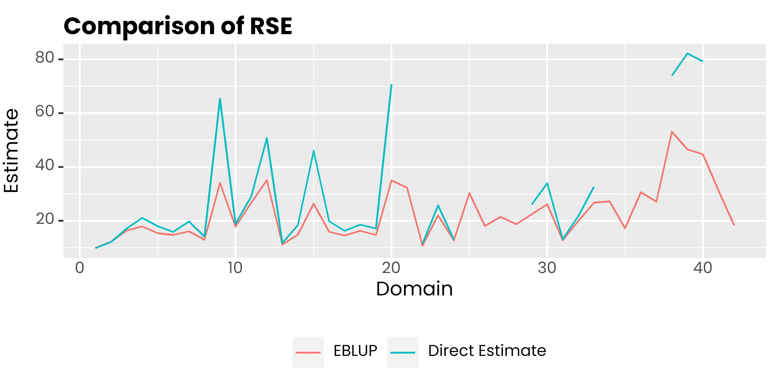
#> $ eblup_rse <dbl> 9.844182, 12.144869, 16.347620, 17.841554, 15.307573, 14.713…

mys %>% 
  select(area, rse, eblup_rse) %>% 
  pivot_longer(-1, names_to = "metode", values_to = "rse") %>%
  ggplot(aes(x = area, y = rse, col = metode)) +
  geom_line() +
    scale_color_discrete(
    labels = c('EBLUP', 'Direct Estimate')
  ) +
  labs(col = NULL, y = 'Estimate', x = 'Domain', title = 'Comparison of RSE') +
  theme(
    legend.position = 'bottom',
    text = element_text(family = 'poppins'),
    axis.ticks.x = element_blank(),
    plot.title = element_text(face = 2, vjust = 0),
    plot.subtitle = element_text(colour = 'gray30', vjust = 0)
  )

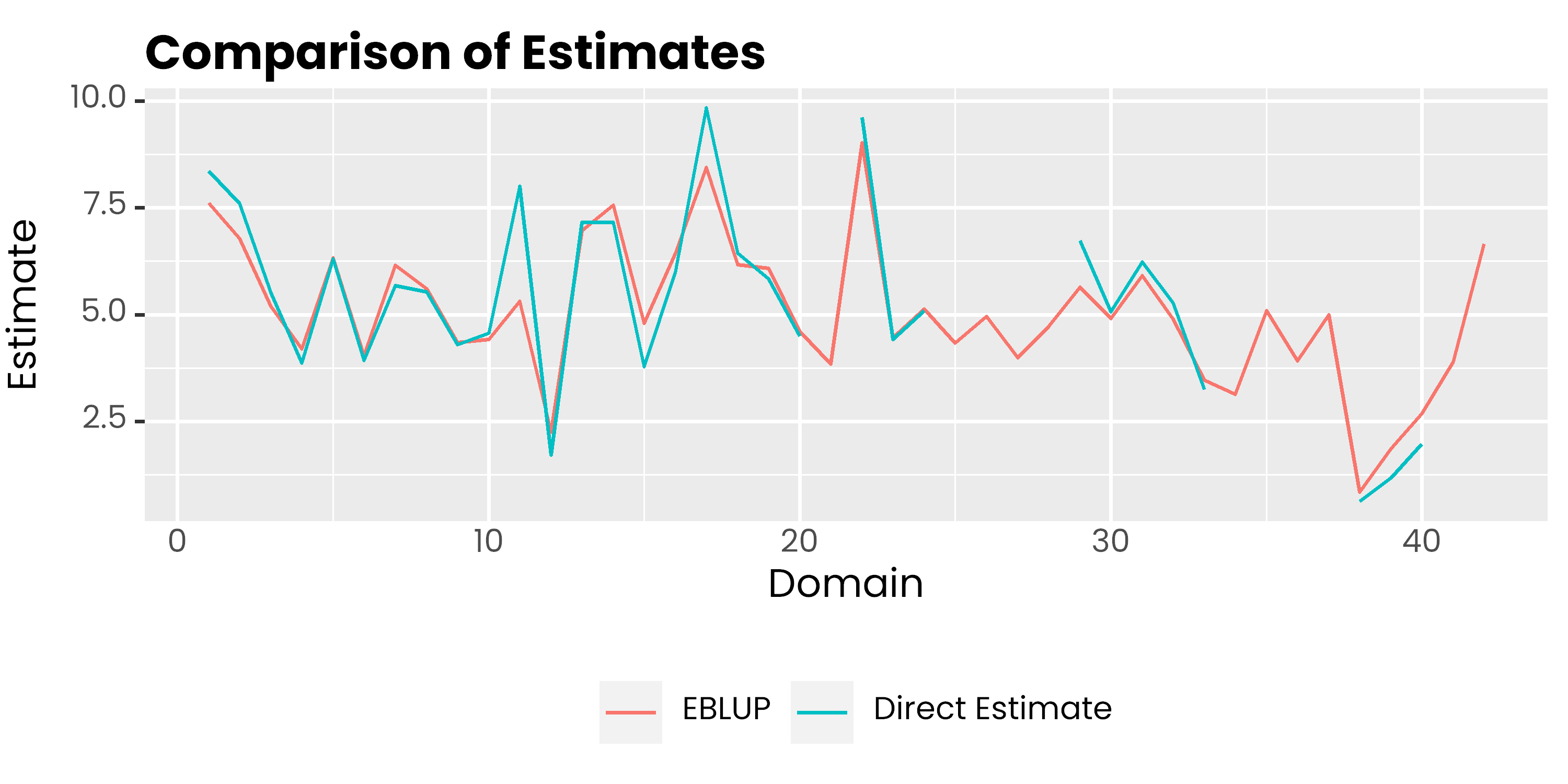
mys %>% 
  select(area, y, eblup_est) %>% 
  pivot_longer(-1, names_to = "metode", values_to = "rse") %>%
  ggplot(aes(x = area, y = rse, col = metode)) +
  geom_line() +
    scale_color_discrete(
    labels = c('EBLUP', 'Direct Estimate')
  ) +
  labs(col = NULL, y = 'Estimate', x = 'Domain', title = 'Comparison of Estimates') +
  theme(
    legend.position = 'bottom',
    text = element_text(family = 'poppins'),
    axis.ticks.x = element_blank(),
    plot.title = element_text(face = 2, vjust = 0),
    plot.subtitle = element_text(colour = 'gray30', vjust = 0)
  )

References

• Rao, J. N., & Molina, I. (2015). Small area estimation. John Wiley & Sons.
• Anisa, R., Kurnia, A., & Indahwati, I. (2013). Cluster information of non-sampled area in small area estimation. E-Prosiding Internasional| Departemen Statistika FMIPA Universitas Padjadjaran, 1(1), 69-76.

These binaries (installable software) and packages are in development.
They may not be fully stable and should be used with caution. We make no claims about them.
Health stats visible at Monitor.