The hardware and bandwidth for this mirror is donated by dogado GmbH, the Webhosting and Full Service-Cloud Provider. Check out our Wordpress Tutorial.
If you wish to report a bug, or if you are interested in having us mirror your free-software or open-source project, please feel free to contact us at mirror[@]dogado.de.
Some Additional Distributions apparently not available in R.
– Steven E. Pav, shabbychef@gmail.com
This package can be installed from CRAN, via drat, or from github:
# via CRAN:
install.packages("sadists")
# via drat:
if (require(drat)) {
    drat:::add("shabbychef")
    install.packages("sadists")
}
# via devtools (typically 'master' is stable):
if (require(devtools)) {
    install_github("shabbychef/sadists")
}First some functions to test the ‘dpqr’ functions:
testf <- function(dpqr, nobs, ...) {
    require(ggplot2)
    require(grid)

    set.seed(3940071)
    rv <- sort(dpqr$r(nobs, ...))
    data <- data.frame(draws = rv, pvals = dpqr$p(rv,
        ...))
    text.size <- 8  # sigh

    # http://stackoverflow.com/a/5688125/164611
    p1 <- ggplot(data, aes(x = draws)) + geom_line(aes(y = ..density..,
        colour = "Empirical"), stat = "density") +
        stat_function(fun = function(x) {
            dpqr$d(x, ...)
        }, aes(colour = "Theoretical")) + geom_histogram(aes(y = ..density..),
        alpha = 0.3) + scale_colour_manual(name = "Density",
        values = c("red", "blue")) + theme(text = element_text(size = text.size)) +
        labs(title = "Density (tests dfunc)")

    # Q-Q plot
    p2 <- ggplot(data, aes(sample = draws)) + stat_qq(distribution = function(p) {
        dpqr$q(p, ...)
    }) + geom_abline(slope = 1, intercept = 0, colour = "red") +
        theme(text = element_text(size = text.size)) +
        labs(title = "Q-Q plot (tests qfunc)")

    # empirical CDF of the p-values; should be uniform
    p3 <- ggplot(data, aes(sample = pvals)) + stat_qq(distribution = qunif) +
        geom_abline(slope = 1, intercept = 0, colour = "red") +
        theme(text = element_text(size = text.size)) +
        labs(title = "P-P plot (tests pfunc)")

    # Define grid layout to locate plots and print each
    # graph
    pushViewport(viewport(layout = grid.layout(2, 2)))
    print(p1, vp = viewport(layout.pos.row = 1, layout.pos.col = 1:2))
    print(p2, vp = viewport(layout.pos.row = 2, layout.pos.col = 1))
    print(p3, vp = viewport(layout.pos.row = 2, layout.pos.col = 2))
}This distribution is the weighted sum of independent (non-central) chi-square variates taken to some powers. The special case where the powers are all one half is related to the upsilon distribution. The special case where the powers are all one could be used to compute the distribution of the (doubly non-central) F distribution.
require(sadists)
wts <- c(-1, 1, 3, -3)
df <- c(100, 200, 100, 50)
ncp <- c(0, 1, 0.5, 2)
pow <- c(1, 0.5, 2, 1.5)
testf(list(d = dsumchisqpow, p = psumchisqpow, q = qsumchisqpow,
    r = rsumchisqpow), nobs = 2^14, wts, df, ncp, pow)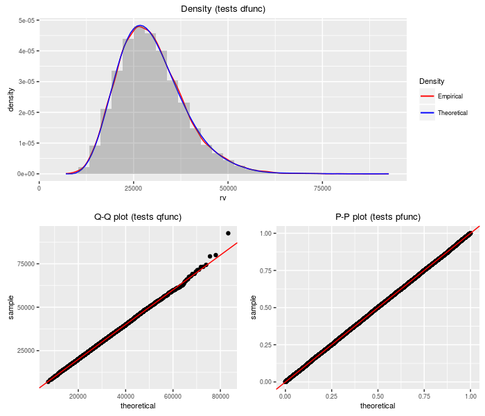
The K-prime distribution is the weighted sum of a standard normal and an independent central chi, all divided by another independent central chi. Depending on the degrees of freedom and the weights, the K-prime can appears as a Lambda-prime, a normal, or a central t.
require(sadists)
v1 <- 50
v2 <- 80
a <- 0.5
b <- 1.5
testf(list(d = dkprime, p = pkprime, q = qkprime, r = rkprime),
    nobs = 2^14, v1, v2, a, b)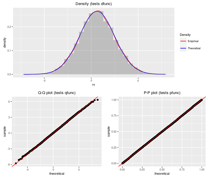
A Lambda prime random variable is the sum of a standard normal and an independent, scaled central chi random variable.
require(sadists)
df <- 70
ts <- 2
testf(list(d = dlambdap, p = plambdap, q = qlambdap,
    r = rlambdap), nobs = 2^14, df, ts)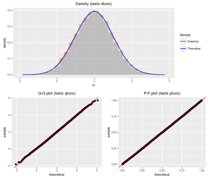
An upsilon random variable is the sum of a standard normal and the weighted sum of several indpendent central chis.
require(sadists)
df <- c(30, 50, 100, 20, 10)
ts <- c(-3, 2, 5, -4, 1)
testf(list(d = dupsilon, p = pupsilon, q = qupsilon,
    r = rupsilon), nobs = 2^14, df, ts)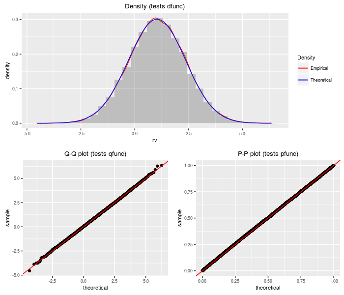
The doubly non-central t distribution generalizes the t distribution to the case where the denominator chi-square is non-central.
require(sadists)
df <- 75
ncp1 <- 2
ncp2 <- 3
testf(list(d = ddnt, p = pdnt, q = qdnt, r = rdnt),
    nobs = 2^14, df, ncp1, ncp2)
The doubly non-central F distribution generalizes the F distribution to the case where the denominator chi-square is non-central.
require(sadists)
df1 <- 40
df2 <- 80
ncp1 <- 1.5
ncp2 <- 2.5
testf(list(d = ddnf, p = pdnf, q = qdnf, r = rdnf),
    nobs = 2^14, df1, df2, ncp1, ncp2)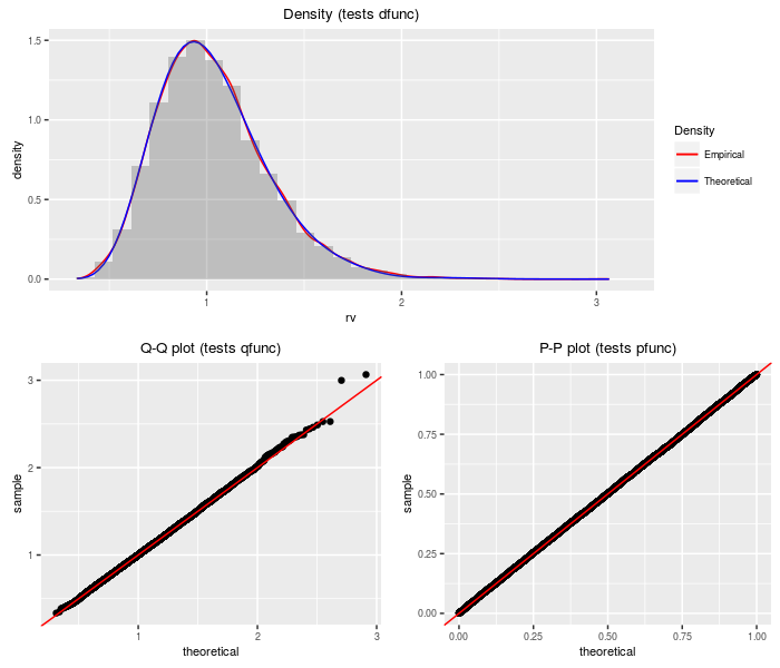
The doubly non-central Beta distribution can be viewed as a transformation of the doubly non-central F distribution.
require(sadists)
df1 <- 40
df2 <- 80
ncp1 <- 1.5
ncp2 <- 2.5
testf(list(d = ddnbeta, p = pdnbeta, q = qdnbeta, r = rdnbeta),
    nobs = 2^14, df1, df2, ncp1, ncp2)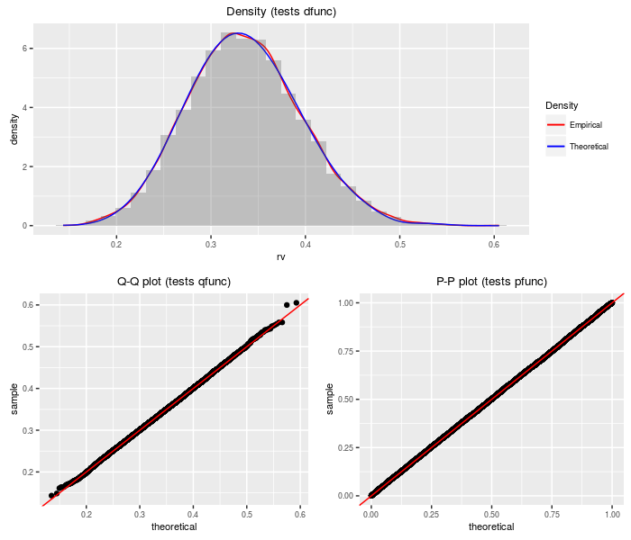
The doubly non-central Eta distribution can be viewed as the square root of the doubly non-central Beta distribution. It is a transform of the doubly non-central t distribution.
require(sadists)
df <- 100
ncp1 <- 0.5
ncp2 <- 2.5
testf(list(d = ddneta, p = pdneta, q = qdneta, r = rdneta),
    nobs = 2^14, df, ncp1, ncp2)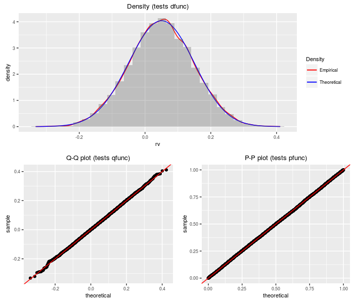
This distribution is the weighted sum of logs of independent (non-central) chi-square variates.
require(sadists)
wts <- c(5, -4, 10, -15)
df <- c(100, 200, 100, 50)
ncp <- c(0, 1, 0.5, 2)
testf(list(d = dsumlogchisq, p = psumlogchisq, q = qsumlogchisq,
    r = rsumlogchisq), nobs = 2^14, wts, df, ncp)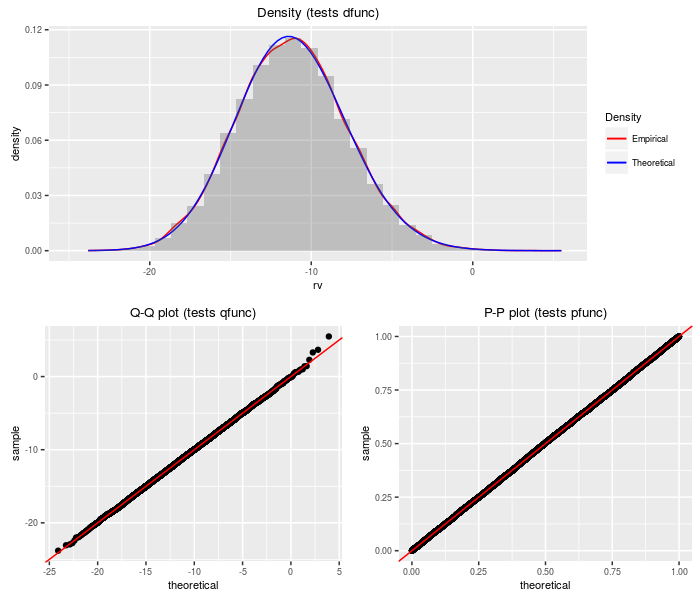
This distribution is the product of independent doubly non-central F variates. The PDQ functions are computed by transformation on the sum of log chi-squares distribution.
require(sadists)
df1 <- c(10, 20, 5)
df2 <- c(1000, 500, 150)
ncp1 <- c(1, 0, 2.5)
ncp2 <- c(0, 1.5, 5)
testf(list(d = dproddnf, p = pproddnf, q = qproddnf,
    r = rproddnf), nobs = 2^14, df1, df2, ncp1, ncp2)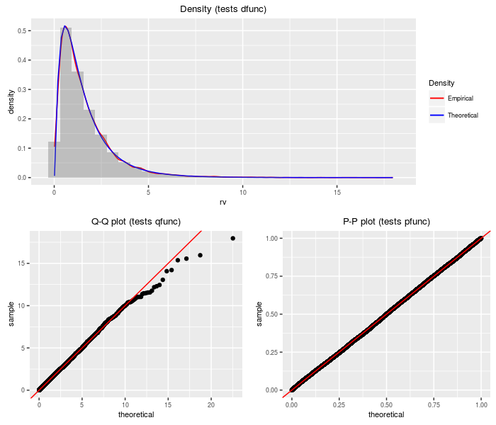
This distribution is the product of independent (non-central) chi-square variates taken to some powers. The PDQ functions are computed by transformation on the sum of log chi-squares distribution.
require(sadists)
df <- c(100, 200, 100, 50)
ncp <- c(0, 1, 0.5, 2)
pow <- c(1, 0.5, 2, 1.5)
testf(list(d = dprodchisqpow, p = pprodchisqpow, q = qprodchisqpow,
    r = rprodchisqpow), nobs = 2^14, df, ncp, pow)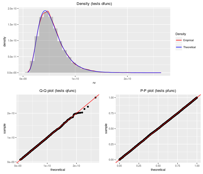
This distribution is the product of independent normal variates. Warning: when the coefficient of variation is large for some of the factors, this approximation can be terrible.
require(sadists)
mu <- c(100, -50, -10)
sigma <- c(10, 5, 10)
testf(list(d = dprodnormal, p = pprodnormal, q = qprodnormal,
    r = rprodnormal), nobs = 2^14, mu, sigma)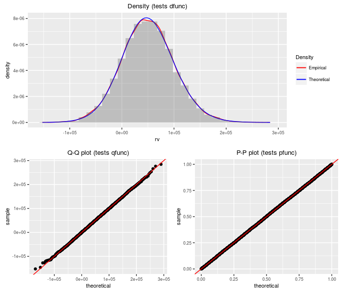
These binaries (installable software) and packages are in development.
They may not be fully stable and should be used with caution. We make no claims about them.
Health stats visible at Monitor.