The hardware and bandwidth for this mirror is donated by dogado GmbH, the Webhosting and Full Service-Cloud Provider. Check out our Wordpress Tutorial.
If you wish to report a bug, or if you are interested in having us mirror your free-software or open-source project, please feel free to contact us at mirror[@]dogado.de.
rkaf is an R package for Kolmogorov-Arnold
Fourier Networks using the torch backend.
The package provides a modern R interface for KAF models, including:
The goal of rkaf is to make KAF-style neural networks
accessible to R users without requiring Python, reticulate,
or custom training loops.
You can install the development version locally with:
devtools::install()Or from a local package directory:
devtools::load_all()rkaf depends on torch. If
torch is not already configured, run:
torch::install_torch()library(rkaf)
set.seed(123)
torch::torch_manual_seed(123)
x <- as.matrix(seq(-1, 1, length.out = 128))
y <- sin(8 * pi * x) +
0.35 * cos(3 * pi * x) +
0.15 * x^2
fit <- kaf_fit(
x = x,
y = y,
hidden = c(256, 256),
num_grids = 32,
use_layernorm = FALSE,
epochs = 1000,
lr = 1e-3,
standardize_x = FALSE,
standardize_y = TRUE,
fourier_init_scale = 5e-2,
restore_best = TRUE,
verbose = FALSE,
seed = 123
)
fit
#> <kaf_fit>
#> Task: regression
#> Architecture: 1 -> 256 -> 256 -> 1
#> Fourier grids: 32
#> Epochs: 1000
#> Batch size: 128
#> Validation: no
#> Standardize x: no
#> Standardize y: yes
#> Final train loss: 0.0227977
#> Best train loss: 0.0198582 at epoch 945pred <- predict(fit, x)
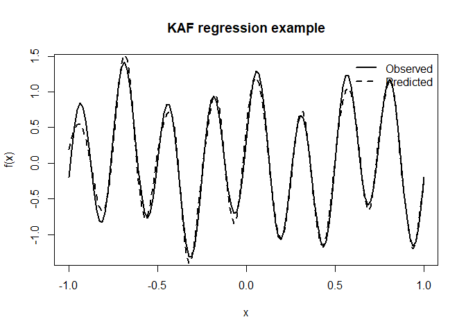
plot(
x,
y,
type = "l",
lwd = 2,
xlab = "x",
ylab = "f(x)",
main = "KAF regression example"
)
lines(x, pred, lwd = 2, lty = 2)
legend(
"topright",
legend = c("Observed", "Predicted"),
lty = c(1, 2),
lwd = 2,
bty = "n"
)
plot(fit)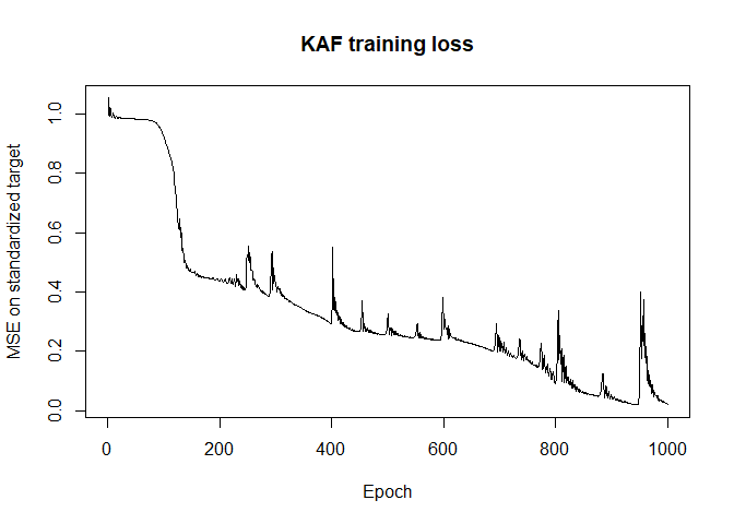
This example intentionally uses a Fourier-heavy target function to demonstrate the model’s ability to learn oscillatory structure.
rkaf also supports a formula interface for tabular
data.
fit_mtcars <- kaf_fit_formula(
  mpg ~ wt + hp + cyl,
  data = mtcars,
  hidden = c(32, 32),
  num_grids = 16,
  epochs = 200,
  verbose = FALSE,
  seed = 123
)

fit_mtcars
#> <kaf_fit>
#> Task:         regression
#> Formula:      mpg ~ wt + hp + cyl
#> Architecture: 3 -> 32 -> 32 -> 1
#> Fourier grids: 16
#> Epochs:       200
#> Batch size:   32
#> Validation:   no
#> Standardize x: yes
#> Standardize y: yes
#> Final train loss: 0.0542788
#> Best train loss:  0.0542788 at epoch 200
mtcars_pred <- predict(fit_mtcars, mtcars)
head(data.frame(
observed = mtcars$mpg,
predicted = round(mtcars_pred, 2)
))
#> observed predicted
#> 1 21.0 21.16
#> 2 21.0 21.15
#> 3 22.8 21.86
#> 4 21.4 20.03
#> 5 18.7 16.58
#> 6 18.1 18.30For factor, character, or logical targets with two classes,
rkaf can fit a binary classifier automatically.
df <- mtcars
df$high_mpg <- factor(
  ifelse(df$mpg > median(df$mpg), "yes", "no"),
  levels = c("no", "yes")
)

fit_binary <- kaf_fit_formula(
  high_mpg ~ wt + hp + cyl,
  data = df,
  hidden = c(32, 32),
  num_grids = 16,
  epochs = 200,
  verbose = FALSE,
  seed = 123
)

fit_binary
#> <kaf_fit>
#> Task:         binary
#> Classes:      no, yes
#> Formula:      high_mpg ~ wt + hp + cyl
#> Architecture: 3 -> 32 -> 32 -> 1
#> Fourier grids: 16
#> Epochs:       200
#> Batch size:   32
#> Validation:   no
#> Standardize x: yes
#> Standardize y: no
#> Final train loss: 0.00163561
#> Best train loss:  0.00163561 at epoch 200
Predicted probabilities and class:
prob_binary <- predict(fit_binary, df, type = "prob")
class_binary <- predict(fit_binary, df, type = "class")

head(data.frame(
  observed = df$high_mpg,
  prob_yes = round(prob_binary, 3),
  predicted = class_binary
))
#>   observed prob_yes predicted
#> 1      yes    0.999       yes
#> 2      yes    0.999       yes
#> 3      yes    1.000       yes
#> 4      yes    0.983       yes
#> 5       no    0.000        no
#> 6       no    0.008        no

table(
  observed = df$high_mpg,
  predicted = class_binary
)
#>         predicted
#> observed no yes
#>      no  17   0
#> yes 0 15For factor targets with more than two classes, rkaf fits
a multiclass model.
fit_iris <- kaf_fit_formula(
  Species ~ .,
  data = iris,
  hidden = c(32, 32),
  num_grids = 16,
  epochs = 300,
  verbose = FALSE,
  seed = 123
)

fit_iris
#> <kaf_fit>
#> Task:         multiclass
#> Classes:      setosa, versicolor, virginica
#> Formula:      Species ~ .
#> Architecture: 4 -> 32 -> 32 -> 3
#> Fourier grids: 16
#> Epochs:       300
#> Batch size:   150
#> Validation:   no
#> Standardize x: yes
#> Standardize y: no
#> Final train loss: 0.00819381
#> Best train loss:  0.00819381 at epoch 300
Class probabilities:
head(round(predict(fit_iris, iris, type = "prob"), 3))
#>      setosa versicolor virginica
#> [1,]  0.999      0.001     0.000
#> [2,]  0.995      0.003     0.002
#> [3,]  0.997      0.001     0.001
#> [4,]  0.997      0.001     0.001
#> [5,]  0.999      0.000     0.000
#> [6,]  1.000      0.000     0.000
Predicted classes:
class_iris <- predict(fit_iris, iris, type = "class")

table(
  observed = iris$Species,
  predicted = class_iris
)
#>             predicted
#> observed     setosa versicolor virginica
#>   setosa         50          0         0
#>   versicolor      0         50         0
#> virginica 0 0 50kaf_fit() supports validation splits, mini-batching, and
early stopping.
fit_val <- kaf_fit(
  x = x,
  y = y,
  hidden = c(64, 64),
  num_grids = 16,
  use_layernorm = FALSE,
  epochs = 300,
  lr = 5e-4,
  batch_size = 64,
  validation_split = 0.2,
  patience = 100,
  restore_best = TRUE,
  verbose = FALSE,
  seed = 123
)

fit_val$train_loss_history
fit_val$validation_loss_history
The fitted object stores both training and validation loss histories,
so users can inspect them directly through
fit_val$train_loss_history and
fit_val$validation_loss_history. The code above is shown as
an example and is not run when building this README.
You can inspect the learned balance between the base/GELU branch and the Fourier branch.
scales <- extract_kaf_scales(fit)
head(scales)
#>   layer feature base_scale fourier_scale fourier_to_base_ratio
#> 1     1       1  1.0369691    0.11137812            0.10740737
#> 2     2       1  0.9652719    0.15750510            0.16317174
#> 3     2       2  0.9738784    0.39944243            0.41015638
#> 4     2       3  0.9945174    0.12360517            0.12428658
#> 5     2       4  0.9936960    0.08714252            0.08769535
#> 6     2       5  1.0083405    0.08873361            0.08799965
fourier_params <- extract_fourier_params(fit, layer = 1)
head(fourier_params)
#> layer input_feature grid weight bias
#> 1 1 1 1 0.1379520 4.5462580
#> 2 1 1 2 -0.1811931 4.3979001
#> 3 1 1 3 -0.1297648 5.7381864
#> 4 1 1 4 -0.4164377 2.7132401
#> 5 1 1 5 0.3679259 0.4899397
#> 6 1 1 6 0.3606938 2.3420620Advanced users can directly create KAF torch modules.
model <- nn_kaf(
  layers = c(4, 16, 16, 1),
  num_grids = 8
)

x_tensor <- torch::torch_randn(10, 4)
y_tensor <- model(x_tensor)

y_tensor$shape
#> [1] 10 1The package currently includes:
devtools::test()
devtools::check()
with full test coverage for the core API, including regression, binary classification, multiclass classification, formula handling, prediction, training utilities, and diagnostics.
rkaf is an independent R implementation of
Kolmogorov-Arnold Fourier Networks using the torch
backend.
The package is based on the KAF architecture proposed in:
Zhang, J., Fan, Y., Cai, K., & Wang, K. (2025).
Kolmogorov-Arnold Fourier Networks.
arXiv:2502.06018.
The implementation was also informed by the public Python reference implementations:
kolmogorovArnoldFourierNetwork/KAFkolmogorovArnoldFourierNetwork/kaf_actNo Python dependency is required by rkaf.
MIT.
These binaries (installable software) and packages are in development.
They may not be fully stable and should be used with caution. We make no claims about them.
Health stats visible at Monitor.