The hardware and bandwidth for this mirror is donated by dogado GmbH, the Webhosting and Full Service-Cloud Provider. Check out our Wordpress Tutorial.
If you wish to report a bug, or if you are interested in having us mirror your free-software or open-source project, please feel free to contact us at mirror[@]dogado.de.
realTimeloads provides tools to compute estimates of analyte flux and load from estimated timeseries of analyte concentration and discharge. An “analyte” is any laboratory measured quantity. Discharge is water volume per unit time. In hydrology timeseries estimates of analyte concentration are often computed as analyte analysis is cost-prohibitive for continuous water-quality monitoring. A synthetic data set is provided to allow users to explore package functionality and to implement all methods detailed in Livsey (in review)
You can install the development version from GitHub with:
# install.packages("devtools")
# devtools::install_github("dlivsey/realTimeloads")This is a basic example which shows how to load data from csv files and compute suspended-sediment loads from an acoustic Doppler velocity meter (ADVM). Data formatted to match the package csv data files can be used to compute loads from user-provided data.
Users are encouraged to explore package functionality via: vignette(“realTimeloads”,package=“realTimeloads”) and ?realTimeLoads. Additional worked examples are provided in realTimeloads::ExampleCode() and realTimeloads::ExampleCodeSCI()
A published example using the package methods can be found in: Livsey et al (2020) https://doi.org/10.1007/s12237-020-00734-z
### Call package and process data ----
library(realTimeloads)
#> Registered S3 method overwritten by 'quantmod':
#>   method            from
#>   as.zoo.data.frame zoo
Input <- realTimeloads::import_data()
Output <- realTimeloads::hADCPLoads(Input)

### Plot results ----
time <- Output$time
Analyte_flux_timeseries_kt <- Output$Analyte_flux_timeseries_kt
# compute dt (seconds) for used for computing load
dt =  c()
dt[2:length(time)] <- as.numeric(difftime(time[2:length(time)],time[1:length(time)-1],units = "secs"))
dt[1] = median(dt,na.rm=TRUE) # assume time step 1 using median dt

Qspt <- Input$Sediment_Samples$SSCpt_mg_per_liter*
Input$Discharge$Discharge_m_cubed_per_s*dt*1e-9 # actual load (kt) from synthetic data

# samples used in regression of analyte(surrogate)
ind <- is.element(time,Output$regression_data$time)

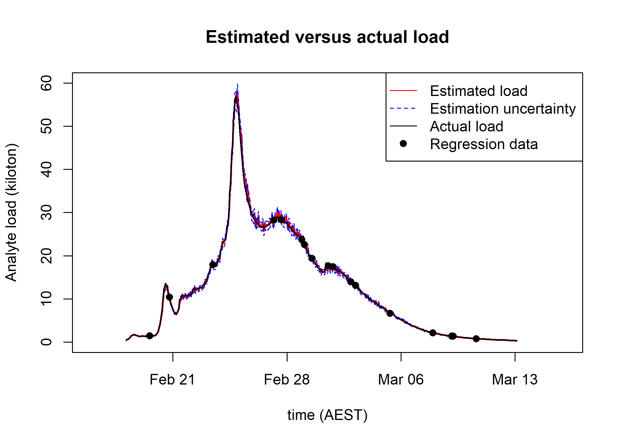
plot(time,Analyte_flux_timeseries_kt$median_confidence,
     col='red',type = "l",lwd= 2,xlab = "time (AEST)",ylab="Analyte load (kiloton)",
     main = "Estimated versus actual load",ylim = c(0,60))
lines(time,Analyte_flux_timeseries_kt$minus_two_sigma_confidence,
      col='blue',lty = c(2))
lines(time,Analyte_flux_timeseries_kt$plus_two_sigma_confidence,
      col='blue',lty = c(2))
lines(time,Qspt,col = 'black',lwd= 1.5)
points(time[ind],Analyte_flux_timeseries_kt$median_confidence[ind],pch = 19)
legend("topright",legend = c("Estimated load","Estimation uncertainty","Actual load","Regression data"),
       lty = c(1,2,1,-1),col = c('red', 'blue', 'black','black'),pch = c(-1,-1,-1,19))
Livsey, D. N., Downing-Kunz, M. A., Schoellhamer, D. H., & Manning, A. J. (2020). Suspended sediment flux in the San Francisco Estuary: Part I—Changes in the vertical distribution of suspended sediment and bias in estuarine sediment flux measurements. Estuaries and Coasts, 43, 1956-1972.
Livsey, D. N., Turner, R. D. R., & Grace, P. R. (2023). Combining Optical and Acoustic Backscatter Measurements for Monitoring of Fine Suspended‐Sediment Concentration Under Changes in Particle Size and Density. Water Resources Research, 59(8), e2022WR033982.
Livsey, D.N. (in review). National Industry Guidelines for hydrometric monitoring–Part 12: Application of acoustic Doppler velocity meters to measure suspended-sediment load. Bureau of Meteorology. Melbourne, Australia
These binaries (installable software) and packages are in development.
They may not be fully stable and should be used with caution. We make no claims about them.
Health stats visible at Monitor.