The hardware and bandwidth for this mirror is donated by dogado GmbH, the Webhosting and Full Service-Cloud Provider. Check out our Wordpress Tutorial.
If you wish to report a bug, or if you are interested in having us mirror your free-software or open-source project, please feel free to contact us at mirror[@]dogado.de.

raem

raem is an R package for modeling steady-state, single-layer groundwater flow under the Dupuit-Forchheimer assumption using analytic elements.

Installation

To install the released version:

install.packages("raem")

The development version of raem can be installed from GitHub with:

# install.packages("devtools")
devtools::install_github("cneyens/raem")

Documentation

The package documentation can be found at https://cneyens.github.io/raem/.

Example

Construct an analytic element model of an aquifer with uniform background flow, two extraction wells and a reference point.

Specify the aquifer parameters and create the elements:

library(raem)

# aquifer parameters ----
k = 10     # hydraulic conductivity, m/d
top = 10   # aquifer top elevation, m
base = 0   # aquifer bottom elevation, m
n = 0.2    # aquifer porosity, -

hr = 15    # head at reference point, m
TR = k * (top - base) # constant transmissivity of background flow, m^2/d

# create elements ----
uf = uniformflow(TR, gradient = 0.001, angle = -45)
rf = constant(xc = -1000, yc = 0, hc = hr)
w1 = well(xw = 200, yw = 0, Q = 250)
w2 = well(xw = -200, yw = -150, Q = 400)

Create the model. This automatically solves the system of equations.

m = aem(k = k, top = top, base = base, n = n, uf, rf, w1, w2)

Find the head and discharge at two locations: x = -200, y = 200 and x = 100, y = 200. Note that there are no vertical flow components in this model:

heads(m, x = c(-200, 100), y = 200)
#> [1] 13.64573 13.33314

discharge(m, c(-200, 100), 200, z = top) # m^2/d
#>              Qx         Qy Qz
#> [1,] 0.15028815 -0.2923908  0
#> [2,] 0.06041242 -0.3347206  0

Plot the head contours and element locations. First, specify the contouring grid:

xg = seq(-500, 500, length = 100)
yg = seq(-250, 250, length = 100)

Now plot:

contours(m, xg, yg, 'heads', col = 'dodgerblue', nlevels = 20)
plot(m, add = TRUE)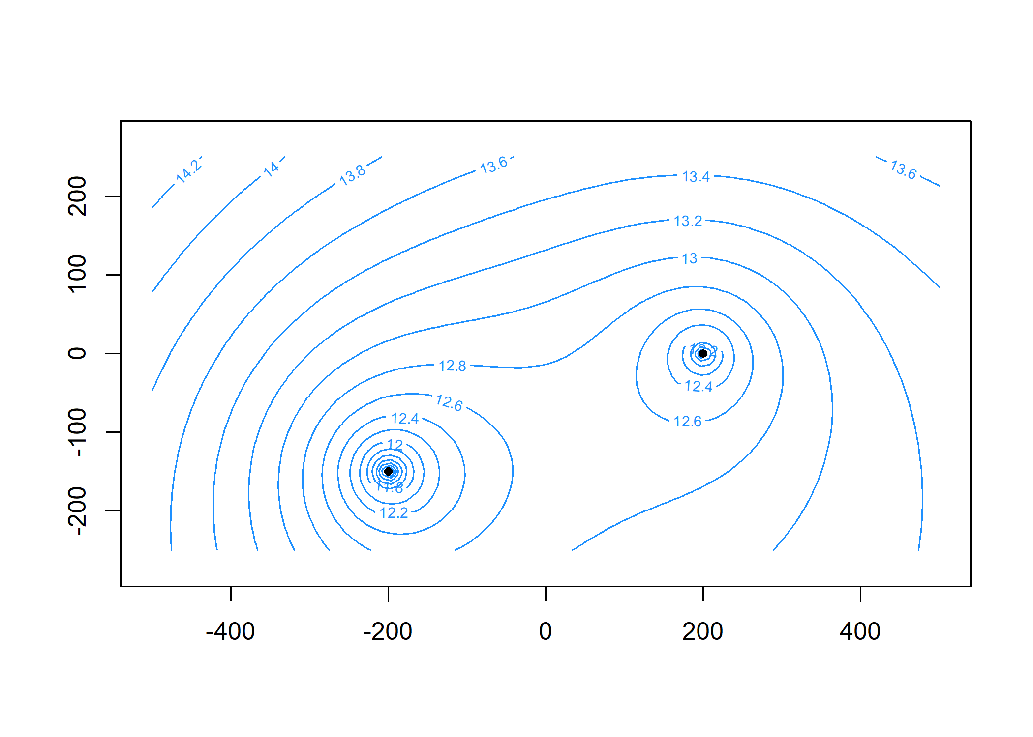

Compute particle traces starting along y = 200 at 20 intervals per year for 5 years and add to the plot:

paths = tracelines(m, 
                   x0 = seq(-450, 450, 50), 
                   y0 = 200, 
                   z0 = top, 
                   times = seq(0, 5 * 365, 365 / 20))

plot(paths, add = TRUE, col = 'orange')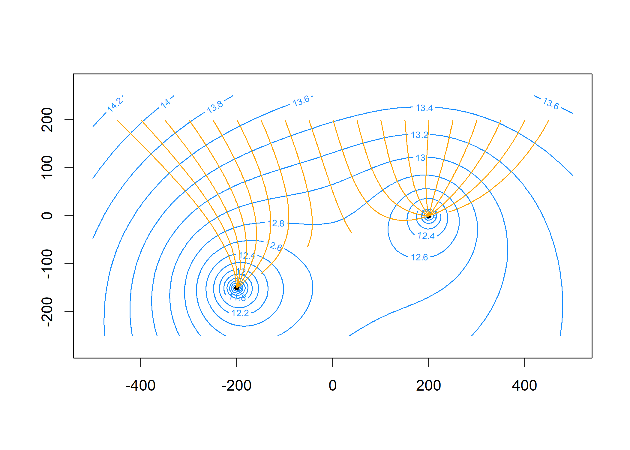

These binaries (installable software) and packages are in development.
They may not be fully stable and should be used with caution. We make no claims about them.
Health stats visible at Monitor.