The hardware and bandwidth for this mirror is donated by dogado GmbH, the Webhosting and Full Service-Cloud Provider. Check out our Wordpress Tutorial.
If you wish to report a bug, or if you are interested in having us mirror your free-software or open-source project, please feel free to contact us at mirror[@]dogado.de.
This package is developed for 3D radial visualization of high-dimensional datasets. Our display engine is called RadViz3D and extends the classic 2D radial visualization and displays multivariate data on the 3D space by mapping every record to a point inside the unit sphere. RadViz3D obtains equi-spaced anchor points exactly for the five Platonic solids and approximately for the other cases via a Fibonacci grid. We also propose a Max-Ratio Projection (MRP) method that utilizes the group information in high dimensions to provide distinctive lower-dimensional projections that are then displayed using Radviz3D. Our methodology is extended to datasets with discrete and mixed features where a generalized distributional transform (GDT) is used in conjuction with copula models before applying MRP and RadViz3D visualization. This document gives a brief introduction to the functions included in radviz3d with several application examples.
The 3D interative plots are implemented with the rgl
functions and here are instructions for manipulation: - Rotation: Click
and hold with the left mouse button, then drag the plot to rotate it and
gain different perspectives. - Resize: Zoom in and out with the scroll
wheel, or the right mouse button.
radviz3d contains 3 functions:
Gtrans: Transform discrete or mixture of discrete and
continuous datasets to continuous datasets with marginal
normal(0,1).mrp: Project high-dimensional datasets to lower
dimention with max-ratio projection.radialvis3d: Visualize appropriately tranformed
datasets in the unit sphere.The main function radialvis3d is able to displays and
classifies data points from the pre-known groups and provide visual
clues to how the grouped data are separately from each other.
We illustrate the usage of radialvis3d on datasets with
small (< 10) and large dimensions and with continuous or discrete
features. The interactive 3D plot are produced from rgl and
can be rotated manually to get better perspectives on
rgl-supported devices.
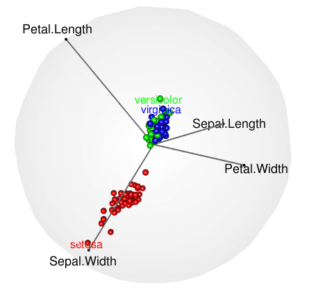
For small datasets with continuous values, function
radialvis3d can be applied directly with options
domrp = F and doGtrans = F. The 3D
plot below are displayed for the (Fisher’s or Anderson’s) iris data. The
dataset contains 50 flowers measurements for 4 variables, sepal length,
sepal width, petal length and petal width which are represented by the 4
anchor points in the plot. Flowers come from each of 3 species, Iris
setosa, Iris versicolor, and Iris virginica. Speicies groups are shown
in different colors and tagged with name labels.
library(radviz3d)
data("iris")
radialvis3d(data = iris[, -5], cl = factor(iris$Species), domrp = F, doGtrans = F,
lwd = 2, alpha = 0.05, pradius = 0.025, class.labels = levels(iris$Species))For large datasets with continuous values, we use function
radialvis3d with options doGtrans = F and
domrp = T along with the number of principal components
k specified by npc = k. The plot for a wine
dataset are shown below. The dataset (reference link: ) contains 178
samples of three types of wines grown in a specific area of Italy. 13
chemical analyses were recorded for each sample.
radialvis3d(data = wine[, -14], cl = factor(wine[,14]), domrp = T, npc = 4, doGtrans = F,
            lwd = 2, alpha = 0.05, pradius = 0.025, class.labels = levels(wine[,14]))
#> cumulative variance explained: 0.9913192 1 1 1 1 1 1 1 1 1 1 1 1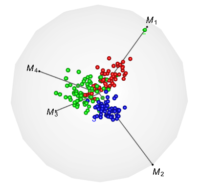
Datasets with discrete values can be transformed using options
doGtrans = T. (Currently, GDT is not applicable to
categorical variables). Here we present an example for an Indic scripts
dataset (reference link: ) which is on 116 different features from
handwritten scripts of 11 Indic languages. A subset of 5 languages is
chosen from 4 regions, namely Bangla (from the east), Gurmukhi (north),
Gujarati (west), and Kannada and Malayalam (languages from the
neighboring southern states of Karnataka and Kerala) and a sixth
language (Urdu, with a distinct Persian script). Some of the features
contains discrete values so the dataset is essentially of mixed
attributes. We apply radialvis3d with GDT and MRP
(npc = 6) to display for distinctiveness of samples
from each languages.
radialvis3d(data = script[,-117], cl = class, domrp = T, npc = 6, doGtrans = T,
            lwd = 2, alpha = 0.05, pradius = 0.025, class.labels = levels(class))
#> cumulative variance explained: 0.3707163 0.6445103 0.8170576 0.9416525 1 1 1 1 1 1 1 1 1 1 1 1 1 1 1 1 1 1 1 1 1 1 1 1 1 1 1 1 1 1 1 1 1 1 1 1 1 1 1 1 1 1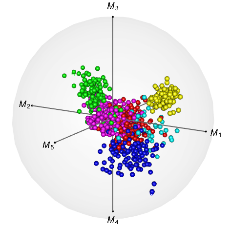
These binaries (installable software) and packages are in development.
They may not be fully stable and should be used with caution. We make no claims about them.
Health stats visible at Monitor.