The hardware and bandwidth for this mirror is donated by dogado GmbH, the Webhosting and Full Service-Cloud Provider. Check out our Wordpress Tutorial.
If you wish to report a bug, or if you are interested in having us mirror your free-software or open-source project, please feel free to contact us at mirror[@]dogado.de.
The goal of rMEA is to provide a suite of tools useful to read, visualize and export bivariate Motion Energy time-series. Lagged synchrony between subjects can be analyzed through windowed cross-correlation. Surrogate data generation allows an estimation of pseudosynchrony that helps to estimate the effect size of the observed synchronization.
This example shows a complete analysis pipeline consisting on Motion Energy time-series import, pre-processing, cross-correlation analysis and comparison between groups against pseudosynchrony.
library(rMEA)
## read the first sample (intake interviews of patients that carried on therapy)
path_normal <- system.file("extdata/normal", package = "rMEA")
mea_normal <- readMEA(path_normal, sampRate = 25, s1Col = 1, s2Col = 2,
s1Name = "Patient", s2Name = "Therapist", skip=1,
idOrder = c("id","session"), idSep="_")
#>
#> STEP 1 | Reading 10 dyads
#> ..................................................|100%
#> ..................................................|Done ;)
#>
#> STEP 2 | Formatting data frames:
#> ..................................................|100%
#> ..................................................|Done ;)
#> Warning: 0.07% of the data was higher than 10 standard deviations in dyad:
#> 200, session: 1, group:all. Check the raw data!
#> Warning: 0.03% of the data was higher than 10 standard deviations in dyad:
#> 201, session: 1, group:all. Check the raw data!
#> Warning: 0.03% of the data was higher than 10 standard deviations in dyad:
#> 202, session: 1, group:all. Check the raw data!
#> Warning: 0.04% of the data was higher than 10 standard deviations in dyad:
#> 204, session: 1, group:all. Check the raw data!
#> Warning: 0.01% of the data was higher than 10 standard deviations in dyad:
#> 205, session: 1, group:all. Check the raw data!
#> Warning: 0.05% of the data was higher than 10 standard deviations in dyad:
#> 206, session: 1, group:all. Check the raw data!
#> Warning: 0.01% of the data was higher than 10 standard deviations in dyad:
#> 208, session: 1, group:all. Check the raw data!
#>
#> STEP 3 | ReadMEA report
#> Filename id_dyad session group duration_hh.mm.ss Patient_%
#> 1 200_01.txt 200 1 all 00:10:00 50.1
#> 2 201_01.txt 201 1 all 00:10:00 50.2
#> 3 202_01.txt 202 1 all 00:10:00 44.6
#> 4 203_01.txt 203 1 all 00:10:00 97.4
#> 5 204_01.txt 204 1 all 00:10:00 66.4
#> 6 205_01.txt 205 1 all 00:10:00 84.3
#> 7 206_01.txt 206 1 all 00:10:00 30.3
#> 8 207_01.txt 207 1 all 00:10:00 52.5
#> 9 208_01.txt 208 1 all 00:10:00 76.6
#> 10 209_01.txt 209 1 all 00:10:00 72.4
#> Therapist_%
#> 1 59.5
#> 2 74.7
#> 3 47.1
#> 4 73.1
#> 5 55.7
#> 6 69.9
#> 7 34.4
#> 8 42.3
#> 9 44.2
#> 10 63.1
mea_normal <- setGroup(mea_normal, "normal")
## read the second sample (intake interviews of patients that dropped out)
path_dropout <- system.file("extdata/dropout", package = "rMEA")
mea_dropout <- readMEA(path_dropout, sampRate = 25, s1Col = 1, s2Col = 2,
s1Name = "Patient", s2Name = "Therapist", skip=1,
idOrder = c("id","session"), idSep="_")
#>
#> STEP 1 | Reading 10 dyads
#> ..................................................|100%
#> ..................................................|Done ;)
#>
#> STEP 2 | Formatting data frames:
#> ..................................................|100%
#> ..................................................|Done ;)
#> Warning: 0.03% of the data was higher than 10 standard deviations in dyad:
#> 100, session: 1, group:all. Check the raw data!
#> Warning: 0.01% of the data was higher than 10 standard deviations in dyad:
#> 101, session: 1, group:all. Check the raw data!
#> Warning: 0.09% of the data was higher than 10 standard deviations in dyad:
#> 104, session: 1, group:all. Check the raw data!
#> Warning: 0.02% of the data was higher than 10 standard deviations in dyad:
#> 105, session: 1, group:all. Check the raw data!
#> Warning: 0.1% of the data was higher than 10 standard deviations in dyad:
#> 106, session: 1, group:all. Check the raw data!
#>
#> STEP 3 | ReadMEA report
#> Filename id_dyad session group duration_hh.mm.ss Patient_%
#> 1 100_01.txt 100 1 all 00:10:00 85.0
#> 2 101_01.txt 101 1 all 00:10:00 84.2
#> 3 102_01.txt 102 1 all 00:10:00 90.9
#> 4 103_01.txt 103 1 all 00:10:00 72.5
#> 5 104_01.txt 104 1 all 00:10:00 72.5
#> 6 105_01.txt 105 1 all 00:10:00 69.2
#> 7 106_01.txt 106 1 all 00:10:00 76.7
#> 8 107_01.txt 107 1 all 00:10:00 95.4
#> 9 108_01.txt 108 1 all 00:10:00 80.1
#> 10 109_01.txt 109 1 all 00:10:00 85.0
#> Therapist_%
#> 1 97.2
#> 2 88.0
#> 3 95.1
#> 4 90.7
#> 5 73.9
#> 6 83.5
#> 7 66.1
#> 8 79.5
#> 9 96.5
#> 10 87.3
mea_dropout <- setGroup(mea_dropout, "dropout")
## Combine into a single object
mea_all <- c(mea_normal, mea_dropout)
summary(mea_all)
#>
#> MEA analysis results:
#> dyad session group Patient_% Therapist_%
#> normal_200_1 200 1 normal 50.1 59.5
#> normal_201_1 201 1 normal 50.2 74.7
#> normal_202_1 202 1 normal 44.6 47.1
#> normal_203_1 203 1 normal 97.4 73.1
#> normal_204_1 204 1 normal 66.4 55.7
#> normal_205_1 205 1 normal 84.3 69.9
#> normal_206_1 206 1 normal 30.3 34.4
#> normal_207_1 207 1 normal 52.5 42.3
#> normal_208_1 208 1 normal 76.6 44.2
#> normal_209_1 209 1 normal 72.4 63.1
#> dropout_100_1 100 1 dropout 85.0 97.2
#> dropout_101_1 101 1 dropout 84.2 88.0
#> dropout_102_1 102 1 dropout 90.9 95.1
#> dropout_103_1 103 1 dropout 72.5 90.7
#> dropout_104_1 104 1 dropout 72.5 73.9
#> dropout_105_1 105 1 dropout 69.2 83.5
#> dropout_106_1 106 1 dropout 76.7 66.1
#> dropout_107_1 107 1 dropout 95.4 79.5
#> dropout_108_1 108 1 dropout 80.1 96.5
#> dropout_109_1 109 1 dropout 85.0 87.3
#>
#> Data processing: raw
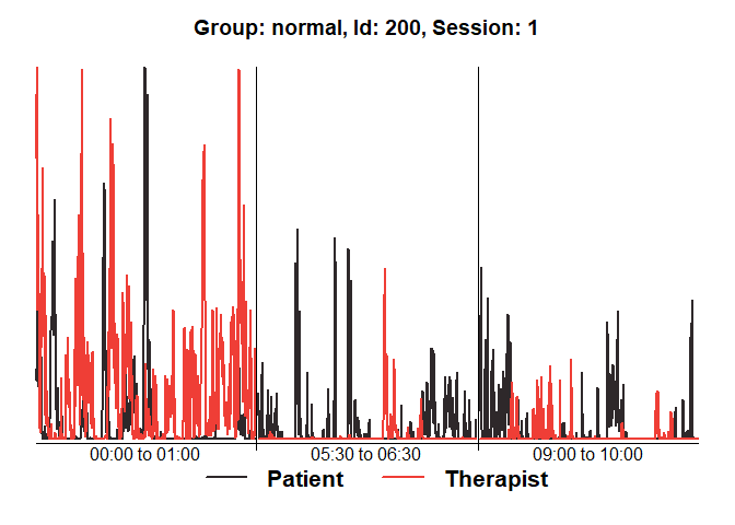
## Show diagnostics for the first session:
diagnosticPlot(mea_all[[1]])
plot(mea_all[[1]], from=1, to=200)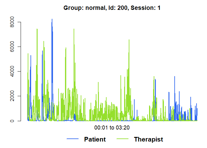
## Filter the data
mea_smoothed <- MEAsmooth(mea_all)
#>
#> Moving average smoothing:
#> ..................................................|100%
#> ..................................................|Done ;)
mea_rescaled <- MEAscale(mea_smoothed)
#>
#> Rescaling data:
#> ..................................................|100%
#> ..................................................|Done ;)

## Generate a random sample
mea_random <- shuffle(mea_rescaled, 50)
#>
#> Shuffling dyads:
#> ..................................................|100%
#> ..................................................|Done ;)
#>
#>  50 / 760 possible combinations were randomly selected

## Run CCF analysis
mea_ccf <- MEAccf(mea_rescaled, lagSec= 5, winSec = 30, incSec=10, ABS = F)
#>
#> Computing CCF:
#> ..................................................|100%
#> ..................................................|Done ;)
mea_random_ccf <- MEAccf(mea_random, lagSec= 5, winSec = 30, incSec=10, ABS = F)
#>
#> Computing CCF:
#> ..................................................|100%
#> ..................................................|Done ;)

## Visualize results

# Raw data of the first session with running lag-0 ccf
plot(mea_ccf[[1]], from=100, to=300, ccf = "lag_zero")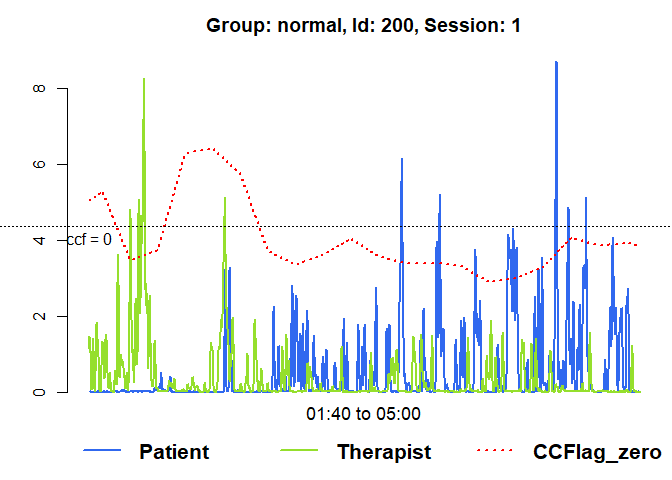
# Heatmap of the first session
MEAheatmap(mea_ccf[[1]])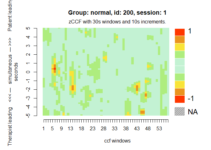
# Distribution of the ccf calculations by group, against random matched dyads
MEAdistplot(mea_ccf, contrast = mea_random_ccf)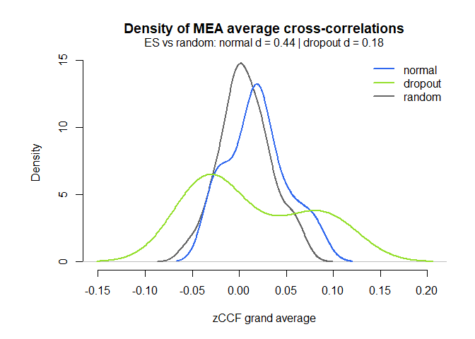
# Representation of the average cross-correlations by lag
MEAlagplot(mea_ccf, contrast=mea_random_ccf)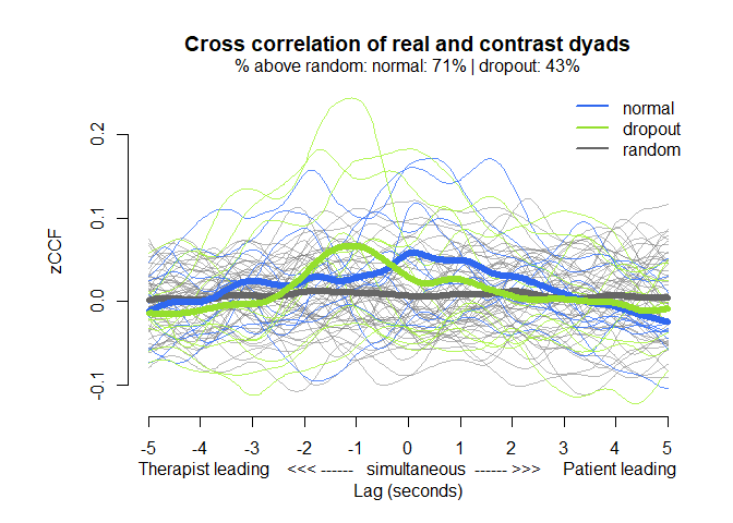
These binaries (installable software) and packages are in development.
They may not be fully stable and should be used with caution. We make no claims about them.
Health stats visible at Monitor.