The hardware and bandwidth for this mirror is donated by dogado GmbH, the Webhosting and Full Service-Cloud Provider. Check out our Wordpress Tutorial.
If you wish to report a bug, or if you are interested in having us mirror your free-software or open-source project, please feel free to contact us at mirror[@]dogado.de.
rEDM is a collection of methods for Empirical Dynamic
Modeling (EDM). EDM is based on the mathematical theory of
reconstructing attractor manifolds from time series data with
applications to forecasting, causal inference, and more. It is based on
research software developed at the Sugihara Lab (University of
California San Diego, Scripps Institution of Oceanography).
Introduction and documentation are are avilable online, or in the package tutorial.
Functionality includes:
To install from CRAN rEDM:
install.packages(rEDM)Using R devtools for latest development version:
install.packages("devtools")
devtools::install_github("SugiharaLab/rEDM")
Building from source:
git clone https://github.com/SugiharaLab/rEDM.git
cd rEDM
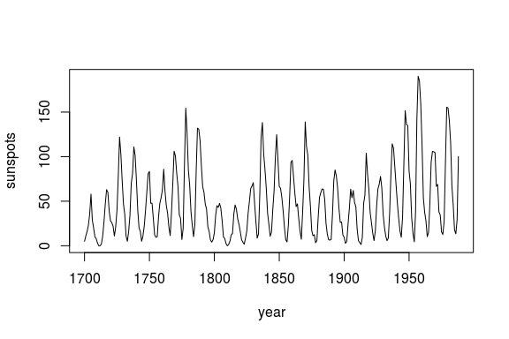
R CMD INSTALL .We begin by looking at annual time series of sunspots:
df = data.frame(yr = as.numeric(time(sunspot.year)),
                 sunspot_count = as.numeric(sunspot.year))

plot(df$yr, df$sunspot_count, type = "l",
     xlab = "year", ylab = "sunspots")
First, we use EmbedDimension() to determine the optimal
embedding dimension, E:
library(rEDM)   # load the package
# If you're new to the rEDM package, please consult the tutorial:
# vignette("rEDM-tutorial")

E.opt = EmbedDimension( dataFrame = df,    # input data
                        lib     = "1 280", # portion of data to train
                        pred    = "1 280", # portion of data to predict
                        columns = "sunspot_count",
                        target  = "sunspot_count" )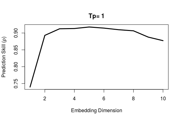
E.opt
#     E    rho
# 1   1 0.7413
# 2   2 0.8954
# 3   3 0.9156
# 4   4 0.9169
# 5   5 0.9207
# 6   6 0.9167
# 7   7 0.9109
# 8   8 0.9078
# 9   9 0.8890
# 10 10 0.8787
E = 3 represents convergence of predictive skill as a
function of E and we use E = 3 to forecast the
last 1/3 of data based on training (attractor reconstruction) from the
first 2/3.
simplex = Simplex( dataFrame = df,
                   lib     = "1   190", # portion of data to train
                   pred    = "191 289", # portion of data to predict
                   columns = "sunspot_count",
                   target  = "sunspot_count",
                   E       = 3 )

plot( df$yr, df$sunspot_count, type = "l", lwd = 2,
      xlab = "year", ylab = "sunspots")
lines( simplex$yr, simplex$Predictions, col = "red", lwd = 2)
legend( 'topleft', legend = c( "Observed", "Predicted (year + 1)" ),
        fill = c( 'black', 'red' ), bty = 'n', cex = 1.3 )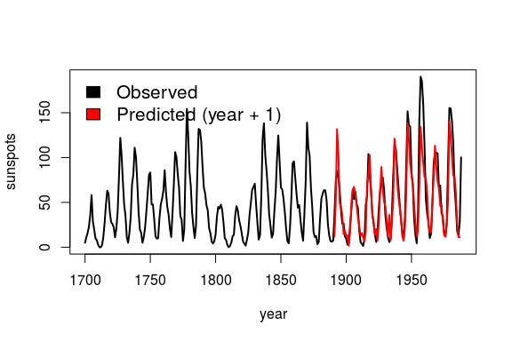
Please see the package vignettes for more details:
browseVignettes("rEDM")Sugihara G. and May R. 1990. Nonlinear forecasting as a way of distinguishing chaos from measurement error in time series. Nature, 344:734–741.
Sugihara G. 1994. Nonlinear forecasting for the classification of natural time series. Philosophical Transactions: Physical Sciences and Engineering, 348 (1688) : 477–495.
Deyle E. R. and Sugihara G. 2011. Generalized theorems for nonlinear state space reconstruction, PLoS One, 6(3) : e18295.
Sugihara G., May R., Ye H., Hsieh C., Deyle E., Fogarty M., Munch S., 2012. Detecting Causality in Complex Ecosystems. Science 338:496-500.
Ye H., and G. Sugihara, 2016. Information leverage in interconnected ecosystems: Overcoming the curse of dimensionality. Science 353:922–925.
These binaries (installable software) and packages are in development.
They may not be fully stable and should be used with caution. We make no claims about them.
Health stats visible at Monitor.