The hardware and bandwidth for this mirror is donated by dogado GmbH, the Webhosting and Full Service-Cloud Provider. Check out our Wordpress Tutorial.
If you wish to report a bug, or if you are interested in having us mirror your free-software or open-source project, please feel free to contact us at mirror[@]dogado.de.

qte — Quantile Treatment Effects in R

Overview

The qte package provides methods for estimating Quantile Treatment Effects (QTE) and Quantile Treatment Effects on the Treated (QTT) in R. Where the average treatment effect summarizes the impact of a policy by a single number, the QTE describes how treatment effects vary across the outcome distribution — useful whenever the policy’s impact is heterogeneous or when distributional consequences (e.g., for inequality) are of interest.

Cross-sectional estimators (no panel data required):

unc_qte() — QTE/QTT under unconfoundedness (IPW, outcome regression, or doubly robust); covers random assignment as a special case

Panel and repeated cross-section estimators (staggered treatment adoption supported for all):

cic() — Change in Changes (Athey and Imbens 2006)
qdid() — Quantile Difference-in-Differences (Athey and Imbens 2006; Meyer, Viscusi, and Durbin 1995)
panel_qtt() — Panel QTT via copula stability (Callaway and Li 2019)
ddid() — Distributional Difference-in-Differences (Callaway and Li
mdid() — Mean Difference-in-Differences (Thuysbaert 2007)
lou_qtt() — Lagged-outcome unconfoundedness QTT

Installation

# Install from CRAN:
install.packages("qte")

# Install the development version from GitHub:
# install.packages("remotes")
remotes::install_github("bcallaway11/qte")

Quick start — unconfoundedness

The unc_qte() function estimates the QTE or QTT under an unconfoundedness assumption. Here we use the observational Lalonde (1986) data to estimate the QTT of a job training program, controlling for pre-treatment characteristics via doubly robust estimation.

data(lalonde)

xf <- ~ age + I(age^2) + education + black + hispanic + married + nodegree

res_cs <- unc_qte(
  yname      = "re78",
  dname      = "treat",
  data       = lalonde.psid,
  xformla    = xf,
  est_method = "aipw",
  target     = "qtt",
  probs      = seq(0.1, 0.9, 0.1),
  biters     = 100
)
summary(res_cs)
#> 
#> Overall ATT:  
#>        ATT    Std. Error     [ 95%  Conf. Int.]  
#>  -4685.583      856.1013  -6363.511   -3007.655 *
#> 
#> 
#> QTT:
#>  Tau         QTT Std. Error [ 95% Simult.  Conf. Band]  
#>  0.1      0.0001    30.0232       -58.8443     58.8444  
#>  0.2  -1002.7420   688.8295     -2352.8229    347.3389  
#>  0.3  -3400.5673  1731.1817     -6793.6212     -7.5135 *
#>  0.4  -5009.2491  1181.6380     -7325.2170  -2693.2811 *
#>  0.5  -4602.4652   848.2877     -6265.0786  -2939.8519 *
#>  0.6  -5229.1454  1230.4344     -7640.7526  -2817.5383 *
#>  0.7  -5507.4720  1199.7046     -7858.8498  -3156.0942 *
#>  0.8  -6885.7529  1376.9064     -9584.4399  -4187.0659 *
#>  0.9 -10517.0625  2373.8362    -15169.6961  -5864.4290 *
#> ---
#> Signif. codes: `*' confidence band does not cover 0

Plot the QTT curve with a uniform confidence band:

autoplot(res_cs)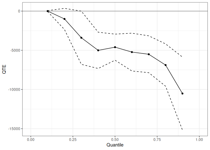

Staggered treatment adoption

All panel estimators use a common yname/gname/tname/idname interface and support staggered treatment adoption via ptetools. The example below uses the mpdta dataset (county-level employment, from the did package) with the Change in Changes estimator.

data(mpdta, package = "did")

res_att <- cic(
  yname   = "lemp",
  gname   = "first.treat",
  tname   = "year",
  idname  = "countyreal",
  data    = mpdta,
  gt_type = "att",
  biters  = 100
)
summary(res_att)
#> 
#> Overall ATT:  
#>      ATT    Std. Error     [ 95%  Conf. Int.] 
#>  -0.0197         0.018    -0.0617      0.0224 
#> 
#> 
#> Dynamic Effects:
#>  Event Time Estimate Std. Error [95% Simult.  Conf. Band]  
#>          -3   0.0508     0.0222        0.0074      0.0943 *
#>          -2   0.0158     0.0147       -0.0130      0.0447  
#>          -1  -0.0128     0.0165       -0.0452      0.0196  
#>           0  -0.0081     0.0171       -0.0416      0.0255  
#>           1  -0.0364     0.0233       -0.0820      0.0092  
#>           2  -0.1226     0.0443       -0.2093     -0.0358 *
#>           3  -0.0930     0.0473       -0.1857     -0.0002 *
#> ---
#> Signif. codes: `*' confidence band does not cover 0

Event-study plot showing pre-trends and post-treatment ATT by event time:

autoplot(res_att, type = "dynamic")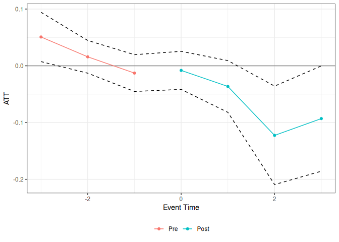

The same estimator returns a full QTT curve when gt_type = "qtt":

res_qtt <- cic(
  yname   = "lemp",
  gname   = "first.treat",
  tname   = "year",
  idname  = "countyreal",
  data    = mpdta,
  gt_type = "qtt",
  probs   = seq(0.1, 0.9, 0.1),
  biters  = 100
)
autoplot(res_qtt)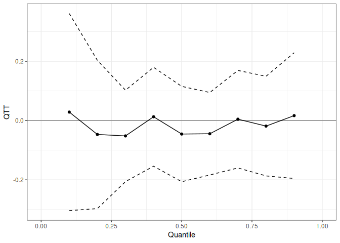

Available estimators

Function	Method	Target	Panel required
`unc_qte()`	Unconfoundedness (IPW / OR / AIPW)	QTE or QTT	No
`cic()`	Change in Changes	ATT or QTT	Optional
`qdid()`	Quantile DiD	ATT or QTT	Optional
`panel_qtt()`	Panel QTT (copula stability)	QTT	Yes
`ddid()`	Distributional DiD	ATT or QTT	Yes
`mdid()`	Mean DiD	ATT or QTT	Optional
`lou_qtt()`	Lagged-outcome unconfoundedness	ATT or QTT	Yes

All panel estimators support staggered treatment adoption and return group-specific, event-study, and overall aggregations.

Documentation and vignettes

Full documentation and vignettes are available at the pkgdown site:

Quantile Treatment Effects in R — unc_qte() under random assignment and selection on observables
Panel Data Estimators for Quantile Treatment Effects — identification assumptions and usage for all six panel estimators
Staggered Treatment Adoption — applied workflow with mpdta: QTT curves, event-study plots, and cross-estimator comparison

These binaries (installable software) and packages are in development.
They may not be fully stable and should be used with caution. We make no claims about them.
Health stats visible at Monitor.