The hardware and bandwidth for this mirror is donated by dogado GmbH, the Webhosting and Full Service-Cloud Provider. Check out our Wordpress Tutorial.
If you wish to report a bug, or if you are interested in having us mirror your free-software or open-source project, please feel free to contact us at mirror[@]dogado.de.
qgcomp v2.18.10
# install developers version (requires devtools)
# install.packages("devtools")
# devtools::install_github("alexpkeil1/qgcomp")     # master version (usually reliable)
# devtools::install_github("alexpkeil1/qgcomp@dev") # dev version (may not be working)
# or install version from CRAN
install.packages("qgcomp")
library("qgcomp")
# using data from the qgcomp package
data("metals", package="qgcomp")

Xnm <- c(
'arsenic','barium','cadmium','calcium','chromium','copper',
'iron','lead','magnesium','manganese','mercury','selenium','silver',
'sodium','zinc'
)

# continuous outcome
results = qgcomp.noboot(y~.,dat=metals[,c(Xnm, 'y')], family=gaussian())
print(results)


> Scaled effect size (positive direction, sum of positive coefficients = 0.39)
>  calcium     iron   barium   silver  arsenic  mercury   sodium chromium  cadmium     zinc
>  0.72216  0.06187  0.05947  0.03508  0.03447  0.02451  0.02162  0.02057  0.01328  0.00696
>
> Scaled effect size (negative direction, sum of negative coefficients = -0.124)
> magnesium    copper      lead manganese  selenium
>  0.475999  0.385299  0.074019  0.063828  0.000857
>
> Mixture slope parameters (Delta method CI):
>
>              Estimate Std. Error Lower CI Upper CI t value  Pr(>|t|)
> (Intercept) -0.356670   0.107878 -0.56811 -0.14523 -3.3062 0.0010238
> psi1         0.266394   0.071025  0.12719  0.40560  3.7507 0.0002001
p = plot(results, suppressprint=TRUE)
ggplot2::ggsave("res1.png", plot=p, dpi=72, width=600/72, height=350/72, units="in")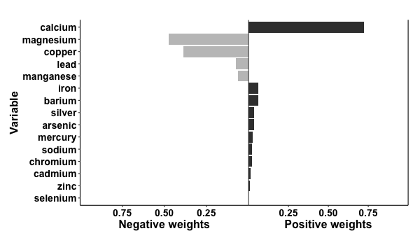
# binary outcome
results2 = qgcomp.noboot(disease_state~., expnms=Xnm,
           data = metals[,c(Xnm, 'disease_state')], family=binomial(), q=4)
print(results2)

> Scaled effect size (positive direction, sum of positive coefficients = 0.392)
>    barium      zinc  chromium magnesium    silver    sodium
>    0.3520    0.2002    0.1603    0.1292    0.0937    0.0645
>
> Scaled effect size (negative direction, sum of negative coefficients = -0.696)
>  selenium    copper   arsenic   calcium manganese   cadmium   mercury      lead      iron
>    0.2969    0.1627    0.1272    0.1233    0.1033    0.0643    0.0485    0.0430    0.0309
>
> Mixture log(OR) (Delta method CI):
>
>             Estimate Std. Error Lower CI Upper CI Z value Pr(>|z|)
> (Intercept)  0.26362    0.51615 -0.74802  1.27526  0.5107   0.6095
> psi1        -0.30416    0.34018 -0.97090  0.36258 -0.8941   0.3713

p2 = plot(results2, suppressprint=TRUE)
ggplot2::ggsave("res2.png", plot=p2, dpi=72, width=600/72, height=350/72, units="in")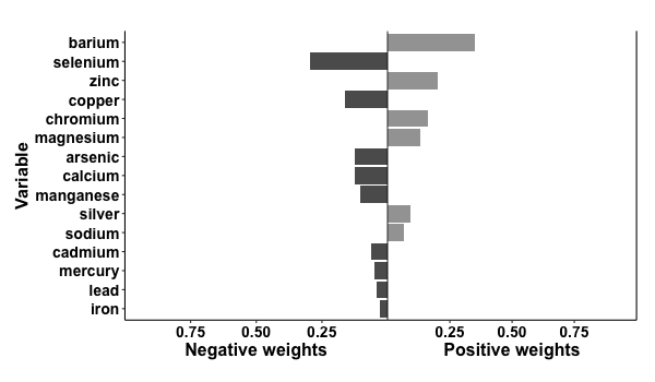
results3 = qgcomp.noboot(y ~ mage35 + arsenic + barium + cadmium + calcium + chloride +
                       chromium + copper + iron + lead + magnesium + manganese +
                       mercury + selenium + silver + sodium + zinc,
                     expnms=Xnm,
                     metals, family=gaussian(), q=4)
print(results3)

> Scaled effect size (positive direction, sum of positive coefficients = 0.381)
>  calcium   barium     iron   silver  arsenic  mercury chromium     zinc   sodium  cadmium
>  0.74466  0.06636  0.04839  0.03765  0.02823  0.02705  0.02344  0.01103  0.00775  0.00543
>
> Scaled effect size (negative direction, sum of negative coefficients = -0.124)
> magnesium    copper      lead manganese  selenium
>   0.49578   0.35446   0.08511   0.06094   0.00372
>
> Mixture slope parameters (Delta method CI):
>
>              Estimate Std. Error Lower CI Upper CI t value  Pr(>|t|)
> (Intercept) -0.348084   0.108037 -0.55983 -0.13634 -3.2219 0.0013688
> psi1         0.256969   0.071459  0.11691  0.39703  3.5960 0.0003601

# coefficient for confounder
results3$fit$coefficients['mage35']
>      mage35
> 0.03463519 results4 = qgcomp.boot(disease_state~., expnms=Xnm,
data = metals[,c(Xnm, 'disease_state')], family=binomial(),
q=4, B=1000,# B should be 200-500+ in practice
seed=125, rr=TRUE)
print(results4)
> Mixture log(RR) (bootstrap CI):
>
> Estimate Std. Error Lower CI Upper CI Z value Pr(>|z|)
> (Intercept) -0.56237 0.23773 -1.02832 -0.096421 -2.3655 0.0180
> psi1 -0.16373 0.17239 -0.50161 0.174158 -0.9497 0.3423
# checking whether model fit seems appropriate (note that the conditional fit
# appears slightly non-linear. The conditional model is on the log-odds scale
# wheras the marginal structural model is on the log-probability scale ).
# The plot is on the log-10 scale.
p4 = plot(results4, suppressprint=TRUE)
ggplot2::ggsave("res4.png", plot=p4, dpi=72, width=600/72, height=350/72, units="in")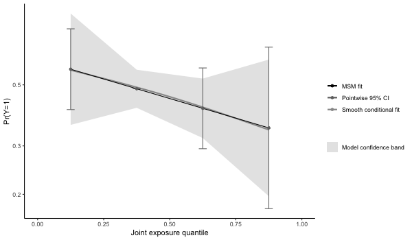
results5 = qgcomp(y~. + .^2 + arsenic*cadmium,
                     expnms=Xnm,
                     metals[,c(Xnm, 'y')], family=gaussian(), q=4, B=10,
                     seed=125, degree=2)

print(results5)

> Mixture slope parameters (bootstrap CI):
>
>             Estimate Std. Error Lower CI Upper CI t value Pr(>|t|)
> (Intercept) -0.89239    0.70336 -2.27095  0.48617 -1.2688   0.2055
> psi1         0.90649    0.93820 -0.93235  2.74533  0.9662   0.3347
> psi2        -0.19970    0.32507 -0.83682  0.43743 -0.6143   0.5395

# some apparent non-linearity, but would require more bootstrap iterations for
# proper test of non-linear mixture effect
p5 = plot(results5, suppressprint=TRUE)
ggplot2::ggsave("res5.png", plot=p5, dpi=72, width=600/72, height=350/72, units="in")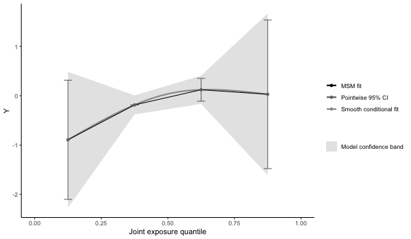
results6 = qgcomp.cox.noboot(Surv(disease_time, disease_state)~.,
                     expnms=Xnm,
                     metals[,c(Xnm, 'disease_time', 'disease_state')])

print(results6)

> Scaled effect size (positive direction, sum of positive coefficients = 0.32)
>    barium      zinc magnesium  chromium    silver    sodium      iron
>    0.3432    0.1946    0.1917    0.1119    0.0924    0.0511    0.0151
>
> Scaled effect size (negative direction, sum of negative coefficients = -0.554)
>  selenium    copper   calcium   arsenic manganese   cadmium      lead   mercury
>    0.2705    0.1826    0.1666    0.1085    0.0974    0.0794    0.0483    0.0466
>
> Mixture log(hazard ratio) (Delta method CI):
>
>      Estimate Std. Error Lower CI Upper CI Z value Pr(>|z|)
> psi1 -0.23356    0.24535 -0.71444  0.24732 -0.9519   0.3411

results7 = qgcomp.cox.boot(Surv(disease_time, disease_state)~.,
                     expnms=Xnm,
                     metals[,c(Xnm, 'disease_time', 'disease_state')],
                     B=10, MCsize=5000)

p7 = plot(results7, suppressprint=TRUE)
ggplot2::ggsave("res7.png", plot=p7, dpi=72, width=600/72, height=350/72, units="in")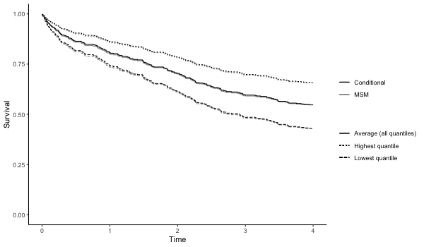
See the vignettes which are included with the qgcomp R
package, and are accessible in R via
vignette("qgcomp-basic-vignette", package="qgcomp") and
vignette("qgcomp-advanced-vignette", package="qgcomp")
Read the original paper: Keil et al. A quantile-based g-computation approach to addressing the effects of exposure mixtures. Env Health Persp. 2019; 128(4)
These binaries (installable software) and packages are in development.
They may not be fully stable and should be used with caution. We make no claims about them.
Health stats visible at Monitor.