The hardware and bandwidth for this mirror is donated by dogado GmbH, the Webhosting and Full Service-Cloud Provider. Check out our Wordpress Tutorial.
If you wish to report a bug, or if you are interested in having us mirror your free-software or open-source project, please feel free to contact us at mirror[@]dogado.de.

publishTC

Why not publish the trend-cycle?

The goal of publishTC is to facilitate the computation, evaluation, and visualization of trend-cycle components from time series using modern state-of-the-art methodology:

Using the Cascade Linear Filter (CLF) and surrogate cut-and-normalise asymmetric filters, as done by Statistics Canada (Dagum and Luati 2008);
Using the classical Henderson symmetric filter and surrogate Musgrave asymmetric filters, as done by the Australian Bureau of Statistics (Trewin 2003);
Using a local parametrization of Musgrave asymmetric filters (Quartier-la-Tente 2024);
Extending Henderson filters to take into account additive outliers (AO) and level shifts (LS) (Quartier-la-Tente 2025).

Installation

To install publishTC:

install.packages('publishTC', repos = c('https://aqlt.r-universe.dev', 'https://cloud.r-project.org'))

Quick Start

library(publishTC)

1. Trend-Cycle Estimation

Estimate the trend-cycle component using the standard Henderson filter:

# Example dataset: French Industrial Production Index
x <- french_ipi[, "manufacturing"]

# Compute Henderson trend-cycle estimates
tc_hend <- henderson_smoothing(x, length = 13)

# Summary diagnostics (I/C ratio, MCD, filter length)
summary(tc_hend)
#> $`I/C ratio`
#> [1] 3.318081
#> 
#> $`I/C ratios`
#>  [1] 3.3180811 1.6933861 1.0927936 0.8358296 0.6684998 0.5812624 0.5760156
#>  [8] 0.5072746 0.4796632 0.4476804 0.4014496 0.4138149
#> 
#> $MCD
#> [1] 4
#> 
#> $Length
#> [1] 13

2. Multi-Method Comparison

Compare different trend-cycle estimation approaches on the same series:

# Estimate trend using multiple methods
all_tc <- smoothing(x)

# Plot comparison
plot(all_tc$henderson, xlim = c(2021, 2024.5))
lines(all_tc$henderson_localic, col_tc = "blue")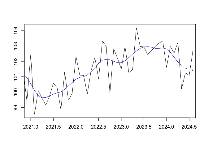

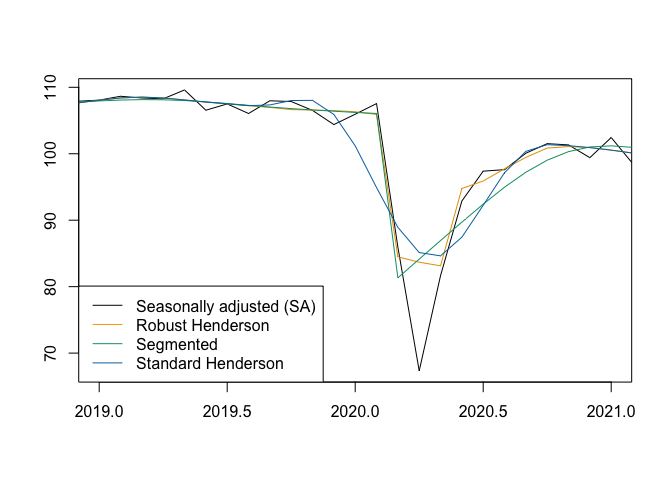
Comparison of trend-cycle estimation methods

3. Outlier-Robust & Segmented Smoothing

Account for Additive Outliers (AO) and Level Shifts (LS) during estimation:

# Identify outliers using RegARIMA wrapper
outliers <- x13_regarima_outliers(x)

# Compute robust Henderson trend-cycle estimates
tc_robust <- henderson_robust_smoothing(
  x, 
  ao = outliers$ao, 
  ls = outliers$ls, 
  local_icr = TRUE
)

# Segmented smoothing around a structural break
tc_seg <- segmented_smoothing(
  x, 
  breaks = list(c(2020, 3)), 
  break_method = "two-sides"
)
plot(tc_robust, xlim = c(2019, 2021))
lines(tc_seg, col_tc = "#009E73")
lines(tc_hend, col_tc = "#0072B2")
legend(
  "bottomleft",
  legend = c(
    "Seasonally adjusted (SA)", "Robust Henderson", 
    "Segmented", "Standard Henderson"
    ),
  col = c("black", "orange", "#009E73", "#0072B2"),
  lty = 1
)

4. Turning Point & Ripple Diagnostics

Identify economic turning points and short-term unwanted ripples:

# Find turning points (upturns and downturns)
tp <- turning_points(tc_hend)
tp
#> $upturn
#>  [1] 1990.667 1991.333 1993.750 1995.833 1998.917 2001.833 2002.833 2003.417
#>  [9] 2004.417 2005.333 2006.583 2007.667 2009.167 2012.833 2013.583 2014.667
#> [17] 2016.333 2018.083 2019.500 2020.250 2021.167 2022.917
#> 
#> $downturn
#>  [1] 1990.917 1991.833 1995.000 1998.417 2001.000 2002.167 2004.167 2004.833
#>  [9] 2006.333 2007.333 2008.000 2011.083 2013.167 2013.917 2015.833 2017.750
#> [17] 2019.083 2019.750 2020.667 2022.583 2023.500
# Count unwanted ripples (cycles under 11 months)
ripples <- unwanted_ripples(tc_hend)
ripples
#> [1] 30

Main Functions Overview

Category	Main Functions
Estimation	`henderson_smoothing()`, `clf_smoothing()`, `henderson_robust_smoothing()`, `segmented_smoothing()`, `smoothing()`
Diagnostics	`icr()`, `icrs()`, `mcd()`, `smoothness()`, `bandwidth()`, `turning_points()`, `unwanted_ripples()`, `implicit_forecasts()`, `underlying_forecasts()`
Visualization (base R)	`plot()`, `lines()`, `lollypop()`, `implicit_forecasts_plot()`, `confint_plot()`, `growthplot()`, `implicit_forecasts_plot()`, `underlying_forecasts_plot()`
Visualization (ggplot2)	`autoplot()`, `gglollypop()`, `ggconfint_plot()`, `ggsmoothing_plot()`, `gggrowthplot()`, `ggimplicit_forecasts_plot()`, `ggunderlying_forecasts_plot()`
Utilities	`write.ts()`, `read.ts()`, `x13_regarima_outliers()`

References

Dagum, E. B., & Luati, A. (2008). A Cascade Linear Filter to Reduce Revisions and False Turning Points for Real Time Trend-Cycle Estimation. Econometric Reviews, 28(1-3), 40‑59. https://doi.org/10.1080/07474930802387837
Henderson, R. (1916). Note on graduation by adjusted average. Transactions of the Actuarial Society of America, 17, 43‑48.
Musgrave, J. (1964). A set of end weights to end all end weights. US Census Bureau [custodian].
Quartier-la-Tente, A. (2024). Improving Real-Time Trend Estimates Using Local Parametrization of Polynomial Regression Filters. Journal of Official Statistics, 40(4), 685-715. https://doi.org/10.1177/0282423X241283207
Quartier-la-Tente, A. (2025). Estimation de la tendance-cycle avec des méthodes robustes aux points atypiques. https://github.com/AQLT/robustMA
Trewin, D. (2003). A guide to interpreting time series - Monitoring trends. Australian Bureau of Statistics Information Paper. https://www.abs.gov.au/AUSSTATS/abs@.nsf/Lookup/1349.0Main+Features12003?OpenDocument

These binaries (installable software) and packages are in development.
They may not be fully stable and should be used with caution. We make no claims about them.
Health stats visible at Monitor.