The hardware and bandwidth for this mirror is donated by dogado GmbH, the Webhosting and Full Service-Cloud Provider. Check out our Wordpress Tutorial.
If you wish to report a bug, or if you are interested in having us mirror your free-software or open-source project, please feel free to contact us at mirror[@]dogado.de.

priorsense

Overview

priorsense provides tools for prior diagnostics and sensitivity analysis.

It currently includes functions for performing power-scaling sensitivity analysis on Stan models. This is a way to check how sensitive a posterior is to perturbations of the prior and likelihood and diagnose the cause of sensitivity. For efficient computation, power-scaling sensitivity analysis relies on Pareto smoothed importance sampling (Vehtari et al., 2024) and importance weighted moment matching (Paananen et al., 2021).

Power-scaling sensitivity analysis and priorsense are described in Kallioinen et al. (2023).

Installation

Download the stable version from CRAN with:

install.packages("priorsense")

Download the development version from GitHub with:

# install.packages("remotes")
remotes::install_github("n-kall/priorsense", ref = "development")

Usage

priorsense works with models created with rstan, cmdstanr or brms, or with draws objects from the posterior package.

Example

Consider a simple univariate model with unknown mu and sigma fit to some data y (available viaexample_powerscale_model("univariate_normal")):

data {
  int<lower=1> N;
  array[N] real y;
}
parameters {
  real mu;
  real<lower=0> sigma;
}
model {
  // priors
  target += normal_lpdf(mu | 0, 1);
  target += normal_lpdf(sigma | 0, 2.5);
  // likelihood
  target += normal_lpdf(y | mu, sigma);
}
generated quantities {
  vector[N] log_lik;
  real lprior;
  // log likelihood
  for (n in 1:N) log_lik[n] =  normal_lpdf(y[n] | mu, sigma);
  // joint log prior
  lprior = normal_lpdf(mu | 0, 1) +
    normal_lpdf(sigma | 0, 2.5);

We first fit the model using Stan:

library(priorsense)

normal_model <- example_powerscale_model("univariate_normal")

fit <- rstan::stan(
  model_code = normal_model$model_code,
  data = normal_model$data,
  refresh = FALSE,
  seed = 123
)

Once fit, sensitivity can be checked as follows:

powerscale_sensitivity(fit)
#> Sensitivity based on cjs_dist:
#> # A tibble: 2 × 4
#>   variable prior likelihood diagnosis          
#>   <chr>    <dbl>      <dbl> <chr>              
#> 1 mu       0.392      0.561 prior-data conflict
#> 2 sigma    0.290      0.530 prior-data conflict

To visually inspect changes to the posterior, use one of the diagnostic plot functions. Estimates with high Pareto-k values may be inaccurate and are indicated.

powerscale_plot_dens(fit)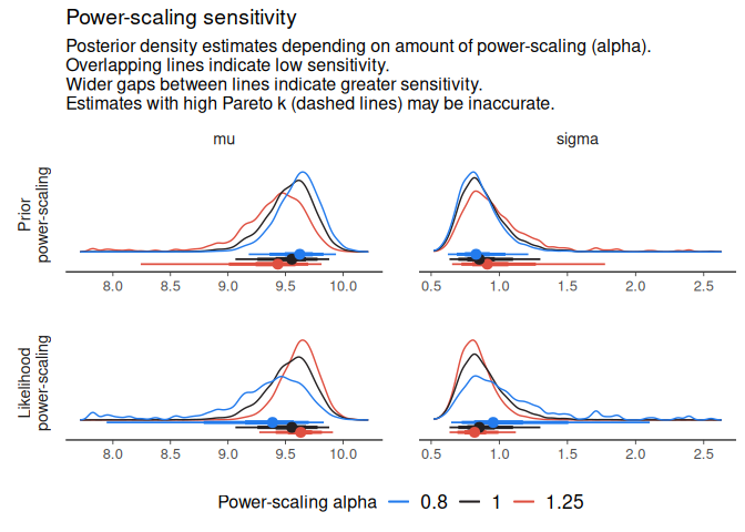

powerscale_plot_ecdf(fit)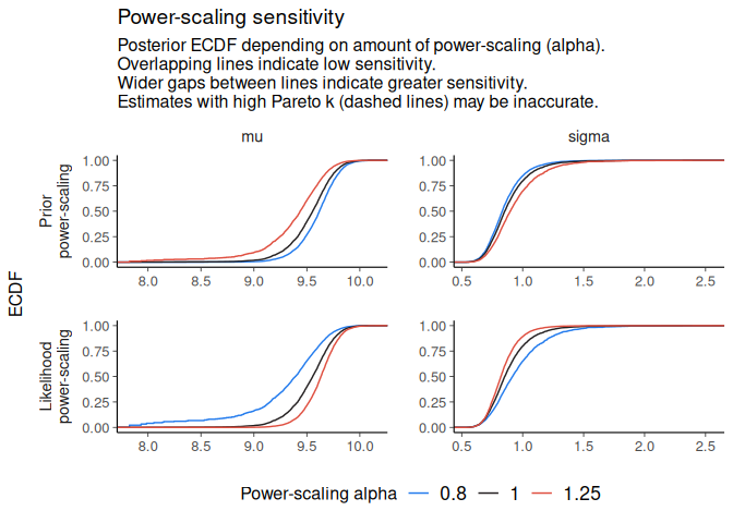

powerscale_plot_quantities(fit)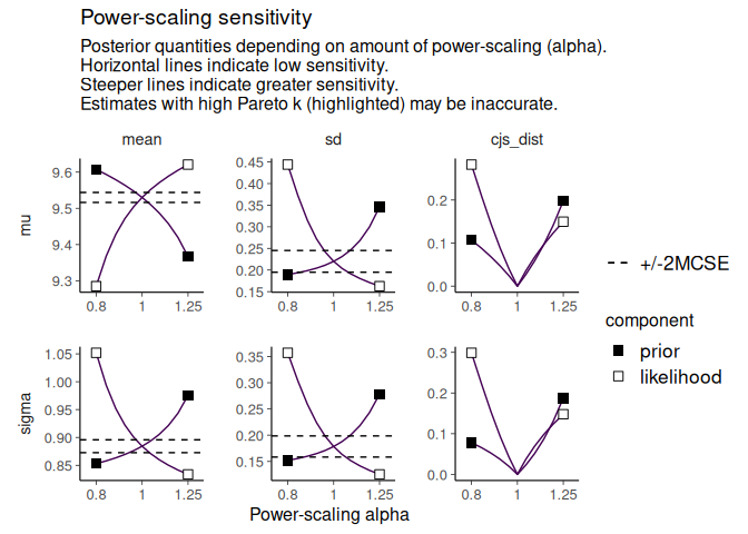

In some cases, setting moment_match = TRUE will improve the unreliable estimates at the cost of some further computation. This requires the iwmm package.

References

Noa Kallioinen, Topi Paananen, Paul-Christian Bürkner, Aki Vehtari (2023). Detecting and diagnosing prior and likelihood sensitivity with power-scaling. Statistics and Computing. 34, 57. https://doi.org/10.1007/s11222-023-10366-5

Topi Paananen, Juho Piironen, Paul-Christian Bürkner, Aki Vehtari (2021). Implicitly adaptive importance sampling. Statistics and Computing 31, 16. https://doi.org/10.1007/s11222-020-09982-2

Aki Vehtari, Daniel Simpson, Andrew Gelman, Yuling Yao, Jonah Gabry (2024). Pareto smoothed importance sampling. Journal of Machine Learning Research. 25, 72. https://jmlr.org/papers/v25/19-556.html

These binaries (installable software) and packages are in development.
They may not be fully stable and should be used with caution. We make no claims about them.
Health stats visible at Monitor.