Title:	Policy Learning
Version:	1.6.0
Description:	Package for learning and evaluating (subgroup) policies via doubly robust loss functions. Policy learning methods include doubly robust blip/conditional average treatment effect learning and sequential policy tree learning. Methods for (subgroup) policy evaluation include doubly robust cross-fitting and online estimation/sequential validation. See Nordland and Holst (2022) <doi:10.48550/arXiv.2212.02335> for documentation and references.
License:	Apache License (≥ 2)
Encoding:	UTF-8
Depends:	R (≥ 4.1), SuperLearner
Imports:	data.table (≥ 1.14.5), lava (≥ 1.7.2.1), future.apply, progressr, methods, policytree (≥ 1.2.0), survival, targeted (≥ 0.6), DynTxRegime
Suggests:	DTRlearn2, glmnet (≥ 4.1-6), mets, mgcv, xgboost, knitr, ranger, rmarkdown, testthat (≥ 3.0), ggplot2
RoxygenNote:	7.3.3
BugReports:	https://github.com/AndreasNordland/polle/issues
VignetteBuilder:	knitr
NeedsCompilation:	no
Packaged:	2025-10-30 12:20:58 UTC; oano
Author:	Andreas Nordland [aut, cre], Klaus Holst [aut]
Maintainer:	Andreas Nordland <andreasnordland@gmail.com>
Repository:	CRAN
Date/Publication:	2025-10-30 13:00:02 UTC

polle: Policy Learning

Description

Package for learning and evaluating (subgroup) policies via doubly robust loss functions. Policy learning methods include doubly robust blip/conditional average treatment effect learning and sequential policy tree learning. Methods for (subgroup) policy evaluation include doubly robust cross-fitting and online estimation/sequential validation. See Nordland and Holst (2022) doi:10.48550/arXiv.2212.02335 for documentation and references.

Author(s)

Maintainer: Andreas Nordland andreasnordland@gmail.com

Authors:

• Klaus Holst klaus@holst.it (ORCID)

See Also

Useful links:

• Report bugs at https://github.com/AndreasNordland/polle/issues

c_model class object

Description

Provides constructors for right-censoring models. Main constructors include:

• c_cox(): Cox proportional hazards model

• c_no_censoring(): Model for scenarios without censoring The constructors are used as input for policy_eval() and policy_learn().

Usage

c_cox(formula = ~., offset = NULL, weights = NULL, ...)

c_no_censoring()

Arguments

Details

c_cox() is a wrapper of mets::phreg() (Cox proportional hazard model).

Value

A c-model object (function) with arguments:

• event: censoring events

• time: start time

• time2: end time

• H: history matrix

See Also

get_history_names().

Conditional Policy Evaluation

Description

conditional() is used to calculate the policy value for each group defined by a given baseline variable.

Usage

conditional(object, policy_data, baseline)

Arguments

Value

object of inherited class 'estimate', see lava::estimate.default. The object is a list with elements 'coef' (policy value estimate for each group) and 'IC' (influence curve estimate matrix).

Examples

library("polle")
library("data.table")
setDTthreads(1)
d <- sim_single_stage(n=2e3)
pd <- policy_data(d,
                  action = "A",
                  baseline = c("B"),
                  covariates = c("Z","L"),
                  utility = "U")

# static policy:
p <- policy_def(1)

pe <- policy_eval(pd,
                  policy = p)

# conditional value for each group defined by B
conditional(pe, pd, "B")

Control arguments for doubly robust blip-learning

Description

control_blip sets the default control arguments for doubly robust blip-learning, type = "blip".

Usage

control_blip(blip_models = q_glm(~.), quantile_prob_threshold = NULL)

Arguments

Value

list of (default) control arguments.

Control arguments for doubly robust Q-learning

Description

control_drql sets the default control arguments for doubly robust Q-learning, type = "drql".

Usage

control_drql(qv_models = q_glm(~.))

Arguments

Value

list of (default) control arguments.

Control arguments for Efficient Augmentation and Relaxation Learning

Description

control_earl sets the default control arguments for efficient augmentation and relaxation learning , type = "earl". The arguments are passed directly to DynTxRegime::earl() if not specified otherwise.

Usage

control_earl(
  moPropen,
  moMain,
  moCont,
  regime,
  iter = 0L,
  fSet = NULL,
  lambdas = 0.5,
  cvFolds = 0L,
  surrogate = "hinge",
  kernel = "linear",
  kparam = NULL,
  verbose = 0L
)

Arguments

Value

list of (default) control arguments.

Control arguments for Outcome Weighted Learning

Description

control_owl() sets the default control arguments for backwards outcome weighted learning, type = "owl". The arguments are passed directly to DTRlearn2::owl() if not specified otherwise.

Usage

control_owl(
  policy_vars = NULL,
  reuse_scales = TRUE,
  res.lasso = TRUE,
  loss = "hinge",
  kernel = "linear",
  augment = FALSE,
  c = 2^(-2:2),
  sigma = c(0.03, 0.05, 0.07),
  s = 2^(-2:2),
  m = 4
)

Arguments

Value

list of (default) control arguments.

Control arguments for Policy Tree Learning

Description

control_ptl sets the default control arguments for doubly robust policy tree learning, type = "ptl". The arguments are passed directly to policytree::policy_tree() (or policytree::hybrid_policy_tree()) if not specified otherwise.

Usage

control_ptl(
  policy_vars = NULL,
  hybrid = FALSE,
  depth = 2,
  search.depth = 2,
  split.step = 1,
  min.node.size = 1
)

Arguments

Value

list of (default) control arguments.

Control arguments for Residual Weighted Learning

Description

control_rwl sets the default control arguments for residual learning , type = "rwl". The arguments are passed directly to DynTxRegime::rwl() if not specified otherwise.

Usage

control_rwl(
  moPropen,
  moMain,
  regime,
  fSet = NULL,
  lambdas = 2,
  cvFolds = 0L,
  kernel = "linear",
  kparam = NULL,
  responseType = "continuous",
  verbose = 2L
)

Arguments

Value

list of (default) control arguments.

Copy Policy Data Object

Description

Objects of class policy_data contains elements of class data.table::data.table. data.table provide functions that operate on objects by reference. Thus, the policy_data object is not copied when modified by reference, see examples. An explicit copy can be made by copy_policy_data. The function is a wrapper of data.table::copy().

Usage

copy_policy_data(object)

Arguments

Value

Object of class policy_data.

Examples

library("polle")
### Single stage case: Wide data
d1 <- sim_single_stage(5e2, seed=1)
head(d1, 5)
# constructing policy_data object:
pd1 <- policy_data(d1,
                   action="A",
                   covariates=c("Z", "B", "L"),
                   utility="U")
pd1

# True copy
pd2 <- copy_policy_data(pd1)
# manipulating the data.table by reference:
pd2$baseline_data[, id := id + 1]
head(pd2$baseline_data$id - pd1$baseline_data$id)

# False copy
pd2 <- pd1
# manipulating the data.table by reference:
pd2$baseline_data[, id := id + 1]
head(pd2$baseline_data$id - pd1$baseline_data$id)

Fit Censoring Functions

Description

Fits right-censoring models for each stage or a single model across all stages.

Usage

fit_c_functions(policy_data, c_models, full_history = FALSE)

Arguments

Details

The function handles two scenarios:

• Multiple models: One model per stage (length K+1)

• Single model: Same model applied across all stages

Value

List of fitted censoring functions with class "c_functions"

Fit g-functions

Description

fit_g_functions is used to fit a list of g-models.

Usage

fit_g_functions(policy_data, g_models, full_history = FALSE)

Arguments

Examples

library("polle")
### Simulating two-stage policy data
d <- sim_two_stage(2e3, seed=1)
pd <- policy_data(d,
                  action = c("A_1", "A_2"),
                  covariates = list(L = c("L_1", "L_2"),
                                    C = c("C_1", "C_2")),
                  utility = c("U_1", "U_2", "U_3"))
pd

# fitting a single g-model across all stages:
g_functions <- fit_g_functions(policy_data = pd,
                               g_models = g_glm(),
                               full_history = FALSE)
g_functions

# fitting a g-model for each stage:
g_functions <- fit_g_functions(policy_data = pd,
                               g_models = list(g_glm(), g_glm()),
                               full_history = TRUE)
g_functions

g_model class object

Description

Use g_glm(), g_empir(), g_glmnet(), g_rf(), g_sl(), g_xgboost to construct an action probability model/g-model object. The constructors are used as input for policy_eval() and policy_learn().

Usage

g_empir(formula = ~1, ...)

g_glm(
  formula = ~.,
  family = "binomial",
  model = FALSE,
  na.action = na.pass,
  ...
)

g_glmnet(formula = ~., family = "binomial", alpha = 1, s = "lambda.min", ...)

g_rf(
  formula = ~.,
  num.trees = c(500),
  mtry = NULL,
  cv_args = list(nfolds = 5, rep = 1),
  ...
)

g_sl(
  formula = ~.,
  SL.library = c("SL.mean", "SL.glm"),
  family = binomial(),
  env = parent.frame(),
  onlySL = TRUE,
  ...
)

g_xgboost(
  formula = ~.,
  objective = "binary:logistic",
  params = list(),
  nrounds,
  max_depth = 6,
  eta = 0.3,
  nthread = 1,
  cv_args = list(nfolds = 3, rep = 1)
)

Arguments

Details

g_glm() is a wrapper of glm() (generalized linear model).
g_empir() calculates the empirical probabilities within the groups defined by the formula.
g_glmnet() is a wrapper of glmnet::glmnet() (generalized linear model via penalized maximum likelihood).
g_rf() is a wrapper of ranger::ranger() (random forest). When multiple hyper-parameters are given, the model with the lowest cross-validation error is selected.
g_sl() is a wrapper of SuperLearner::SuperLearner (ensemble model).
g_xgboost() is a wrapper of xgboost::xgboost.

Value

g-model object: function with arguments 'A' (action vector), 'H' (history matrix) and 'action_set'.

See Also

get_history_names(), get_g_functions().

Examples

library("polle")
### Two stages:
d <- sim_two_stage(2e2, seed=1)
pd <- policy_data(d,
                  action = c("A_1", "A_2"),
                  baseline = c("B"),
                  covariates = list(L = c("L_1", "L_2"),
                                    C = c("C_1", "C_2")),
                  utility = c("U_1", "U_2", "U_3"))
pd

# available state history variable names:
get_history_names(pd)
# defining a g-model:
g_model <- g_glm(formula = ~B+C)

# evaluating the static policy (A=1) using inverse propensity weighting
# based on a state glm model across all stages:
pe <- policy_eval(type = "ipw",
                  policy_data = pd,
                  policy = policy_def(1, reuse = TRUE),
                 g_models = g_model)
# inspecting the fitted g-model:
get_g_functions(pe)

# available full history variable names at each stage:
get_history_names(pd, stage = 1)
get_history_names(pd, stage = 2)

# evaluating the same policy based on a full history
# glm model for each stage:
pe <- policy_eval(type = "ipw",
                   policy_data = pd,
                   policy = policy_def(1, reuse = TRUE),
                   g_models = list(g_glm(~ L_1 + B),
                                   g_glm(~ A_1 + L_2 + B)),
                   g_full_history = TRUE)
# inspecting the fitted g-models:
get_g_functions(pe)

Get Maximal Stages

Description

get_K returns the maximal number of stages for the observations in the policy data object.

Usage

get_K(object)

Arguments

Value

Integer.

Examples

d <- sim_multi_stage(5e2, seed = 1)
pd <- policy_data(data = d$stage_data,
                   baseline_data = d$baseline_data,
                   type = "long",
                   id = "id",
                   stage = "stage",
                   event = "event",
                   action = "A",
                   utility = "U")
pd
# getting the maximal number of stages:
get_K(pd)

Get Action Set

Description

get_action_set returns the action set, i.e., the possible actions at each stage for the policy data object.

Usage

get_action_set(object)

Arguments

Value

Character vector.

Examples

### Two stages:
d <- sim_two_stage(5e2, seed=1)
# constructing policy_data object:
pd <- policy_data(d,
                  action = c("A_1", "A_2"),
                  baseline = c("B"),
                  covariates = list(L = c("L_1", "L_2"),
                                    C = c("C_1", "C_2")),
                  utility = c("U_1", "U_2", "U_3"))
pd

# getting the actions set:
get_action_set(pd)

Get Actions

Description

get_actions returns the actions at every stage for every observation in the policy data object.

Usage

get_actions(object)

Arguments

Value

data.table::data.table with keys id and stage and character variable A.

Examples

### Two stages:
d <- sim_two_stage(5e2, seed=1)
# constructing policy_data object:
pd <- policy_data(d,
                  action = c("A_1", "A_2"),
                  baseline = c("B"),
                  covariates = list(L = c("L_1", "L_2"),
                                    C = c("C_1", "C_2")),
                  utility = c("U_1", "U_2", "U_3"))
pd

# getting the actions:
head(get_actions(pd))

Get event indicators

Description

get_event returns the event indicators for given IDs stages

Usage

get_event(object)

Arguments

Value

data.table::data.table with keys id and stage.

Get g-functions

Description

get_g_functions() returns a list of (fitted) g-functions associated with each stage.

Usage

get_g_functions(object)

Arguments

Value

List of class nuisance_functions.

See Also

predict.nuisance_functions

Examples

### Two stages:
d <- sim_two_stage(5e2, seed=1)
pd <- policy_data(d,
                  action = c("A_1", "A_2"),
                  baseline = c("B"),
                  covariates = list(L = c("L_1", "L_2"),
                                    C = c("C_1", "C_2")),
                  utility = c("U_1", "U_2", "U_3"))
pd

# evaluating the static policy a=1 using inverse propensity weighting
# based on a GLM model at each stage
pe <- policy_eval(type = "ipw",
                  policy_data = pd,
                  policy = policy_def(1, reuse = TRUE, name = "A=1"),
                  g_models = list(g_glm(), g_glm()))
pe

# getting the g-functions
g_functions <- get_g_functions(pe)
g_functions

# getting the fitted g-function values
head(predict(g_functions, pd))

Get history variable names

Description

get_history_names() returns the state covariate names of the history data table for a given stage. The function is useful when specifying the design matrix for g_model and q_model objects.

Usage

get_history_names(object, stage)

Arguments

Value

Character vector.

Examples

library("polle")
### Multiple stages:
d3 <- sim_multi_stage(5e2, seed = 1)
pd3 <- policy_data(data = d3$stage_data,
                   baseline_data = d3$baseline_data,
                   type = "long",
                   id = "id",
                   stage = "stage",
                   event = "event",
                   action = "A",
                   utility = "U")
pd3
# state/Markov type history variable names (H):
get_history_names(pd3)
# full history variable names (H_k) at stage 2:
get_history_names(pd3, stage = 2)

Get IDs

Description

get_id returns the ID for every observation in the policy data object.

Usage

get_id(object)

Arguments

Value

Character vector.

Examples

### Two stages:
d <- sim_two_stage(5e2, seed=1)
# constructing policy_data object:
pd <- policy_data(d,
                  action = c("A_1", "A_2"),
                  baseline = c("B"),
                  covariates = list(L = c("L_1", "L_2"),
                                    C = c("C_1", "C_2")),
                  utility = c("U_1", "U_2", "U_3"))
pd

# getting the IDs:
head(get_id(pd))

Get IDs and Stages

Description

get_id_stage returns the ID and stage number differnt types of events.

Usage

get_id_stage(object, event_set = c(0))

Arguments

Value

data.table::data.table with keys id and stage.

Examples

### Two stages:
d <- sim_two_stage(5e2, seed=1)
# constructing policy_data object:
pd <- policy_data(d,
                  action = c("A_1", "A_2"),
                  baseline = c("B"),
                  covariates = list(L = c("L_1", "L_2"),
                                    C = c("C_1", "C_2")),
                  utility = c("U_1", "U_2", "U_3"))
pd

# getting the IDs and stages:
head(get_id_stage(pd))

Get Number of Observations

Description

get_n returns the number of observations in the policy data object.

Usage

get_n(object)

Arguments

Value

Integer.

Examples

### Two stages:
d <- sim_two_stage(5e2, seed=1)
# constructing policy_data object:
pd <- policy_data(d,
                  action = c("A_1", "A_2"),
                  baseline = c("B"),
                  covariates = list(L = c("L_1", "L_2"),
                                    C = c("C_1", "C_2")),
                  utility = c("U_1", "U_2", "U_3"))
pd

# getting the number of observations:
get_n(pd)

Get Policy

Description

get_policy extracts the policy from a policy object or a policy evaluation object The policy is a function which take a policy data object as input and returns the policy actions.

Usage

get_policy(object, threshold = NULL)

Arguments

Value

function of class policy.

Examples

library("polle")
### Two stages:
d <- sim_two_stage(5e2, seed = 1)
pd <- policy_data(d,
  action = c("A_1", "A_2"),
  baseline = c("BB"),
  covariates = list(
    L = c("L_1", "L_2"),
    C = c("C_1", "C_2")
  ),
  utility = c("U_1", "U_2", "U_3")
)
pd

### V-restricted (Doubly Robust) Q-learning

# specifying the learner:
pl <- policy_learn(
  type = "drql",
  control = control_drql(qv_models = q_glm(formula = ~C))
)

# fitting the policy (object):
po <- pl(
  policy_data = pd,
  q_models = q_glm(),
  g_models = g_glm()
)

# getting and applying the policy:
head(get_policy(po)(pd))

# the policy learner can also be evaluated directly:
pe <- policy_eval(
  policy_data = pd,
  policy_learn = pl,
  q_models = q_glm(),
  g_models = g_glm()
)

# getting and applying the policy again:
head(get_policy(pe)(pd))

Get Policy Actions

Description

get_policy_actions() extract the actions dictated by the (learned and possibly cross-fitted) policy a every stage.

Usage

get_policy_actions(object)

Arguments

Value

data.table::data.table with keys id and stage and action variable d.

Examples

### Two stages:
d <- sim_two_stage(5e2, seed=1)
pd <- policy_data(d,
                  action = c("A_1", "A_2"),
                  covariates = list(L = c("L_1", "L_2"),
                                    C = c("C_1", "C_2")),
                  utility = c("U_1", "U_2", "U_3"))
pd

# defining a policy learner based on cross-fitted doubly robust Q-learning:
pl <- policy_learn(type = "drql",
                   control = control_drql(qv_models = list(q_glm(~C_1), q_glm(~C_1+C_2))),
                   full_history = TRUE,
                   L = 2) # number of folds for cross-fitting

# evaluating the policy learner using 2-fold cross fitting:
pe <- policy_eval(type = "dr",
                   policy_data = pd,
                   policy_learn = pl,
                   q_models = q_glm(),
                   g_models = g_glm(),
                   M = 2) # number of folds for cross-fitting

# Getting the cross-fitted actions dictated by the fitted policy:
head(get_policy_actions(pe))

Get Policy Functions

Description

get_policy_functions() returns a function defining the policy at the given stage. get_policy_functions() is useful when implementing the learned policy.

Usage

## S3 method for class 'blip'
get_policy_functions(
  object,
  stage,
  threshold = NULL,
  include_g_values = FALSE,
  ...
)

## S3 method for class 'drql'
get_policy_functions(
  object,
  stage,
  threshold = NULL,
  include_g_values = FALSE,
  ...
)

get_policy_functions(object, stage, threshold, ...)

## S3 method for class 'ptl'
get_policy_functions(object, stage, threshold = NULL, ...)

## S3 method for class 'ql'
get_policy_functions(
  object,
  stage,
  threshold = NULL,
  include_g_values = FALSE,
  ...
)

Arguments

Value

Functions with arguments:

H

data.table::data.table containing the variables needed to evaluate the policy (and g-function).

Examples

library("polle")
### Two stages:
d <- sim_two_stage(5e2, seed=1)
pd <- policy_data(d,
                  action = c("A_1", "A_2"),
                  baseline = "BB",
                  covariates = list(L = c("L_1", "L_2"),
                                    C = c("C_1", "C_2")),
                  utility = c("U_1", "U_2", "U_3"))
pd

### Realistic V-restricted Policy Tree Learning
# specifying the learner:
pl <- policy_learn(type = "ptl",
                   control = control_ptl(policy_vars = list(c("C_1", "BB"),
                                                            c("L_1", "BB"))),
                   full_history = TRUE,
                   alpha = 0.05)

# evaluating the learner:
pe <- policy_eval(policy_data = pd,
                  policy_learn = pl,
                  q_models = q_glm(),
                  g_models = g_glm())

# getting the policy function at stage 2:
pf2 <- get_policy_functions(pe, stage = 2)
args(pf2)

# applying the policy function to new data:
set.seed(1)
L_1 <- rnorm(n = 10)
new_H <- data.frame(C = rnorm(n = 10),
                    L = L_1,
                    L_1 = L_1,
                    BB = "group1")
d2 <- pf2(H = new_H)
head(d2)

Get Policy Object

Description

Extract the fitted policy object.

Usage

get_policy_object(object)

Arguments

Value

Object of class policy_object.

Examples

library("polle")
### Single stage:
d1 <- sim_single_stage(5e2, seed=1)
pd1 <- policy_data(d1, action="A", covariates=list("Z", "B", "L"), utility="U")
pd1


# evaluating the policy:
pe1 <- policy_eval(policy_data = pd1,
                   policy_learn = policy_learn(type = "drql",
                                               control = control_drql(qv_models = q_glm(~.))),
                   g_models = g_glm(),
                   q_models = q_glm())

# extracting the policy object:
get_policy_object(pe1)

Get Q-functions

Description

get_q_functions() returns a list of (fitted) Q-functions associated with each stage.

Usage

get_q_functions(object)

Arguments

Value

List of class nuisance_functions.

See Also

predict.nuisance_functions

Examples

### Two stages:
d <- sim_two_stage(5e2, seed = 1)
pd <- policy_data(d,
  action = c("A_1", "A_2"),
  baseline = c("B"),
  covariates = list(
    L = c("L_1", "L_2"),
    C = c("C_1", "C_2")
  ),
  utility = c("U_1", "U_2", "U_3")
)
pd

# evaluating the static policy a=1 using outcome regression
# based on a GLM model at each stage.
pe <- policy_eval(
  type = "or",
  policy_data = pd,
  policy = policy_def(1, reuse = TRUE, name = "A=1"),
  q_models = list(q_glm(), q_glm())
)
pe

# getting the Q-functions
q_functions <- get_q_functions(pe)

# getting the fitted g-function values
head(predict(q_functions, pd))

Get Stage Action Sets

Description

get_stage_action_sets returns the action sets at each stage, i.e., the possible actions at each stage for the policy data object.

Usage

get_stage_action_sets(object)

Arguments

Value

List of character vectors.

Examples

### Two stages:
d <- sim_two_stage_multi_actions(5e2, seed=1)
# constructing policy_data object:
pd <- policy_data(d,
                  action = c("A_1", "A_2"),
                  baseline = c("B"),
                  covariates = list(L = c("L_1", "L_2"),
                                    C = c("C_1", "C_2")),
                  utility = c("U_1", "U_2", "U_3"))
pd

# getting the stage actions set:
get_stage_action_sets(pd)

Get the Utility

Description

get_utility() returns the utility, i.e., the sum of the rewards, for every observation in the policy data object.

Usage

get_utility(object)

Arguments

Value

data.table::data.table with key id and numeric variable U.

Examples

### Two stages:
d <- sim_two_stage(5e2, seed=1)
# constructing policy_data object:
pd <- policy_data(d,
                  action = c("A_1", "A_2"),
                  baseline = c("B"),
                  covariates = list(L = c("L_1", "L_2"),
                                    C = c("C_1", "C_2")),
                  utility = c("U_1", "U_2", "U_3"))
pd

# getting the utility:
head(get_utility(pd))

Get History Object

Description

get_history summarizes the history and action at a given stage from a policy_data object.

Usage

get_history(object, stage = NULL, full_history = FALSE, event_set = c(0))

Arguments

Details

Each observation has the sequential form

O= {B, U_1, X_1, A_1, ..., U_K, X_K, A_K, U_{K+1}},

for a possibly stochastic number of stages K.

• B is a vector of baseline covariates.

• U_k is the reward at stage k (not influenced by the action A_k).

• X_k is a vector of state covariates summarizing the state at stage k.

• A_k is the categorical action at stage k.

Value

Object of class history. The object is a list containing the following elements:

Examples

library("polle")
### Single stage:
d1 <- sim_single_stage(5e2, seed=1)
# constructing policy_data object:
pd1 <- policy_data(d1, action="A", covariates=list("Z", "B", "L"), utility="U")
pd1

# In the single stage case, set stage = NULL
h1 <- get_history(pd1)
head(h1$H)
head(h1$A)

### Two stages:
d2 <- sim_two_stage(5e2, seed=1)
# constructing policy_data object:
pd2 <- policy_data(d2,
                  action = c("A_1", "A_2"),
                  baseline = c("B"),
                  covariates = list(L = c("L_1", "L_2"),
                                    C = c("C_1", "C_2")),
                  utility = c("U_1", "U_2", "U_3"))
pd2
# getting the state/Markov-type history across all stages:
h2 <- get_history(pd2)
head(h2$H)
head(h2$A)

# getting the full history at stage 2:
h2 <- get_history(pd2, stage = 2, full_history = TRUE)
head(h2$H)
head(h2$A)
head(h2$U)

# getting the state/Markov-type history at stage 2:
h2 <- get_history(pd2, stage = 2, full_history = FALSE)
head(h2$H)
head(h2$A)

### Multiple stages
d3 <- sim_multi_stage(5e2, seed = 1)
# constructing policy_data object:
pd3 <- policy_data(data = d3$stage_data,
                   baseline_data = d3$baseline_data,
                   type = "long",
                   id = "id",
                   stage = "stage",
                   event = "event",
                   action = "A",
                   utility = "U")
pd3

# getting the full history at stage 2:
h3 <- get_history(pd3, stage = 2, full_history = TRUE)
head(h3$H)
# note that not all observations have two stages:
nrow(h3$H) # number of observations with two stages.
get_n(pd3) # number of observations in total.

Nuisance Functions

Description

The fitted g-functions and Q-functions are stored in an object of class "nuisance_functions". The object is a list with a fitted model object for every stage. Information on whether the full history or the state/Markov-type history is stored as an attribute ("full_history").

S3 generics

The following S3 generic functions are available for an object of class nuisance_functions:

predict

Predict the values of the g- or Q-functions based on a policy_data object.

Examples

### Two stages:
d <- sim_two_stage(5e2, seed=1)
pd <- policy_data(d,
                  action = c("A_1", "A_2"),
                  covariates = list(L = c("L_1", "L_2"),
                                    C = c("C_1", "C_2")),
                  utility = c("U_1", "U_2", "U_3"))
pd

# evaluating the static policy a=1:
pe <- policy_eval(policy_data = pd,
                  policy = policy_def(1, reuse = TRUE),
                  g_models = g_glm(),
                  q_models = q_glm())

# getting the fitted g-functions:
(g_functions <- get_g_functions(pe))

# getting the fitted Q-functions:
(q_functions <- get_q_functions(pe))

# getting the fitted values:
head(predict(g_functions, pd))
head(predict(q_functions, pd))

Trim Number of Stages

Description

partial creates a partial policy data object by trimming the maximum number of stages in the policy data object to a fixed given number.

Usage

partial(object, K)

Arguments

Value

Object of class policy_data.

Examples

library("polle")
### Multiple stage case
d <- sim_multi_stage(5e2, seed = 1)
# constructing policy_data object:
pd <- policy_data(data = d$stage_data,
                   baseline_data = d$baseline_data,
                   type = "long",
                   id = "id",
                   stage = "stage",
                   event = "event",
                   action = "A",
                   utility = "U")
pd
# Creating a partial policy data object with 3 stages
pd3 <- partial(pd, K = 3)
pd3

Plot policy data for given policies

Description

Plot policy data for given policies

Usage

## S3 method for class 'policy_data'
plot(
  x,
  policy = NULL,
  which = c(1),
  stage = 1,
  history_variables = NULL,
  jitter = 0.05,
  ...
)

Arguments

Examples

library("polle")
library("data.table")
setDTthreads(1)
d3 <- sim_multi_stage(2e2, seed = 1)
pd3 <- policy_data(data = d3$stage_data,
                   baseline_data = d3$baseline_data,
                   type = "long",
                   id = "id",
                   stage = "stage",
                   event = "event",
                   action = "A",
                   utility = "U")
pd3 <- partial(pd3, K = 3)

# specifying two static policies:
p0 <- policy_def(c(1,1,0), name = "p0")
p1 <- policy_def(c(1,0,0), name = "p1")

plot(pd3)
plot(pd3, policy = list(p0, p1))

# learning and plotting a policy:
 pe3 <- policy_eval(pd3,
                    policy_learn = policy_learn(),
                    q_models = q_glm(formula = ~t + X + X_lead))
plot(pd3, list(get_policy(pe3), p0))

# plotting the recommended actions at a specific stage:
plot(pd3, get_policy(pe3),
     which = 2,
     stage = 2,
     history_variables = c("t","X"))

Plot histogram of the influence curve for a policy_eval object

Description

Plot histogram of the influence curve for a policy_eval object

Usage

## S3 method for class 'policy_eval'
plot(x, ...)

Arguments

Examples

d <- sim_two_stage(2e3, seed=1)
pd <- policy_data(d,
                  action = c("A_1", "A_2"),
                  baseline = "BB",
                  covariates = list(L = c("L_1", "L_2"),
                                    C = c("C_1", "C_2")),
                  utility = c("U_1", "U_2", "U_3"))

pe <- policy_eval(pd,
                  policy_learn = policy_learn())

plot(pe)

Policy-class

Description

A function of inherited class "policy" takes a policy data object as input and returns the policy actions for every observation for every (observed) stage.

Details

A policy can either be defined directly by the user using policy_def or a policy can be fitted using policy_learn (or policy_eval). policy_learn returns a policy_object from which the policy can be extracted using get_policy.

Value

data.table::data.table with keys id and stage and action variable d.

S3 generics

The following S3 generic functions are available for an object of class policy:

print

Baisc print function

Examples

### Two stages:
d <- sim_two_stage(5e2, seed=1)
pd <- policy_data(d,
                  action = c("A_1", "A_2"),
                  covariates = list(L = c("L_1", "L_2"),
                                    C = c("C_1", "C_2")),
                  utility = c("U_1", "U_2", "U_3"))

# defining a dynamic policy:
p <- policy_def(
  function(L) (L>0)*1,
  reuse = TRUE
)
p
head(p(pd), 5)

# V-restricted (Doubly Robust) Q-learning:
# specifying the learner:
pl <- policy_learn(type = "drql",
                   control = control_drql(qv_models = q_glm(formula = ~ C)))

# fitting the policy (object):
po <- pl(policy_data = pd,
         q_models = q_glm(),
         g_models = g_glm())

p <- get_policy(po)
p

head(p(pd))

Create Policy Data Object

Description

policy_data() creates a policy data object which is used as input to policy_eval() and policy_learn() for policy evaluation and data adaptive policy learning.

Usage

policy_data(
  data,
  baseline_data,
  type = "wide",
  action,
  covariates,
  utility,
  baseline = NULL,
  deterministic_rewards = NULL,
  id = NULL,
  stage = NULL,
  event = NULL,
  time = NULL,
  time2 = NULL,
  action_set = NULL,
  verbose = FALSE
)

## S3 method for class 'policy_data'
print(x, digits = 2, ...)

## S3 method for class 'policy_data'
summary(object, probs = seq(0, 1, 0.25), ...)

Arguments

Details

Each observation has the sequential form

O= {B, U_1, X_1, A_1, ..., U_K, X_K, A_K, U_{K+1}},

for a possibly stochastic number of stages K.

• B is a vector of baseline covariates.

• U_k is the reward at stage k (not influenced by the action A_k).

• X_k is a vector of state covariates summarizing the state at stage k.

• A_k is the categorical action at stage k.

The utility is given by the sum of the rewards, i.e., U = \sum_{k = 1}^{K+1} U_k.

Value

policy_data() returns an object of class "policy_data". The object is a list containing the following elements:

S3 generics

The following S3 generic functions are available for an object of class policy_data:

partial()

Trim the maximum number of stages in a policy_data object.

subset_id()

Subset a a policy_data object on ID.

get_history()

Summarize the history and action at a given stage.

get_history_names()

Get history variable names.

get_actions()

Get the action at every stage.

get_utility()

Get the utility.

plot()

Plot method.

See Also

policy_eval(), policy_learn(), copy_policy_data()

Examples

library("polle")
### Single stage: Wide data
d1 <- sim_single_stage(n = 5e2, seed=1)
head(d1, 5)
# constructing policy_data object:
pd1 <- policy_data(d1,
                   action="A",
                   covariates=c("Z", "B", "L"),
                   utility="U")
pd1
# associated S3 methods:
methods(class = "policy_data")
head(get_actions(pd1), 5)
head(get_utility(pd1), 5)
head(get_history(pd1)$H, 5)

### Two stage: Wide data
d2 <- sim_two_stage(5e2, seed=1)
head(d2, 5)
# constructing policy_data object:
pd2 <- policy_data(d2,
                  action = c("A_1", "A_2"),
                  baseline = c("B"),
                  covariates = list(L = c("L_1", "L_2"),
                                    C = c("C_1", "C_2")),
                  utility = c("U_1", "U_2", "U_3"))
pd2
head(get_history(pd2, stage = 2)$H, 5) # state/Markov type history and action, (H_k,A_k).
head(get_history(pd2, stage = 2, full_history = TRUE)$H, 5) # Full history and action, (H_k,A_k).

### Multiple stages: Long data
d3 <- sim_multi_stage(5e2, seed = 1)
head(d3$stage_data, 10)
# constructing policy_data object:
pd3 <- policy_data(data = d3$stage_data,
                   baseline_data = d3$baseline_data,
                   type = "long",
                   id = "id",
                   stage = "stage",
                   event = "event",
                   action = "A",
                   utility = "U")
pd3
head(get_history(pd3, stage = 3)$H, 5) # state/Markov type history and action, (H_k,A_k).
head(get_history(pd3, stage = 2, full_history = TRUE)$H, 5) # Full history and action, (H_k,A_k).

Define Policy

Description

policy_def returns a function of class policy. The function input is a policy_data object and it returns a data.table::data.table with keys id and stage and action variable d.

Usage

policy_def(policy_functions, full_history = FALSE, reuse = FALSE, name = NULL)

Arguments

Value

Function of class "policy". The function takes a policy_data object as input and returns a data.table::data.table with keys id and stage and action variable d.

See Also

get_history_names(), get_history().

Examples

library("polle")
### Single stage"
d1 <- sim_single_stage(5e2, seed=1)
pd1 <- policy_data(d1, action="A", covariates=list("Z", "B", "L"), utility="U")
pd1

# defining a static policy (A=1):
p1_static <- policy_def(1)

# applying the policy:
p1_static(pd1)

# defining a dynamic policy:
p1_dynamic <- policy_def(
  function(Z, L) ((3*Z + 1*L -2.5)>0)*1
)
p1_dynamic(pd1)

### Two stages:
d2 <- sim_two_stage(5e2, seed = 1)
pd2 <- policy_data(d2,
                  action = c("A_1", "A_2"),
                  covariates = list(L = c("L_1", "L_2"),
                                    C = c("C_1", "C_2")),
                  utility = c("U_1", "U_2", "U_3"))

# defining a static policy (A=0):
p2_static <- policy_def(0,
                        reuse = TRUE)
p2_static(pd2)

# defining a reused dynamic policy:
p2_dynamic_reuse <- policy_def(
  function(L) (L > 0)*1,
  reuse = TRUE
)
p2_dynamic_reuse(pd2)

# defining a dynamic policy for each stage based on the full history:
# available variable names at each stage:
get_history_names(pd2, stage = 1)
get_history_names(pd2, stage = 2)

p2_dynamic <- policy_def(
  policy_functions = list(
    function(L_1) (L_1 > 0)*1,
    function(L_1, L_2) (L_1 + L_2 > 0)*1
  ),
  full_history = TRUE
)
p2_dynamic(pd2)

Policy Evaluation

Description

policy_eval() is used to estimate the value of a given fixed policy or a data adaptive policy (e.g. a policy learned from the data). policy_eval() is also used to estimate the average treatment effect among the subjects who would get the treatment under the policy.

Usage

policy_eval(
  policy_data,
  policy = NULL,
  policy_learn = NULL,
  g_functions = NULL,
  g_models = g_glm(),
  g_full_history = FALSE,
  save_g_functions = TRUE,
  q_functions = NULL,
  q_models = q_glm(),
  q_full_history = FALSE,
  save_q_functions = TRUE,
  c_functions = NULL,
  c_models = NULL,
  c_full_history = FALSE,
  save_c_functions = TRUE,
  m_function = NULL,
  m_model = NULL,
  m_full_history = FALSE,
  save_m_function = TRUE,
  target = "value",
  type = "dr",
  cross_fit_type = "pooled",
  variance_type = "pooled",
  M = 1,
  nrep = 1,
  min_subgroup_size = 1,
  future_args = list(future.seed = TRUE),
  name = NULL
)

## S3 method for class 'policy_eval'
coef(object, ...)

## S3 method for class 'policy_eval'
IC(x, ...)

## S3 method for class 'policy_eval'
vcov(object, ...)

## S3 method for class 'policy_eval'
print(
  x,
  digits = 4L,
  width = 35L,
  std.error = TRUE,
  level = 0.95,
  p.value = TRUE,
  ...
)

## S3 method for class 'policy_eval'
summary(object, ...)

## S3 method for class 'policy_eval'
estimate(
  x,
  labels = get_element(x, "name", check_name = FALSE),
  level = 0.95,
  ...
)

## S3 method for class 'policy_eval'
merge(x, y, ..., paired = TRUE)

## S3 method for class 'policy_eval'
x + ...

## S3 method for class 'policy_eval_online'
vcov(object, ...)

Arguments

Details

Each observation has the sequential form

O= {B, U_1, X_1, A_1, ..., U_K, X_K, A_K, U_{K+1}},

for a possibly stochastic number of stages K.

• B is a vector of baseline covariates.

• U_k is the reward at stage k (not influenced by the action A_k).

• X_k is a vector of state covariates summarizing the state at stage k.

• A_k is the categorical action within the action set \mathcal{A} at stage k.

The utility is given by the sum of the rewards, i.e., U = \sum_{k = 1}^{K+1} U_k.

A policy is a set of functions

d = \{d_1, ..., d_K\},

where d_k for k\in \{1, ..., K\} maps \{B, X_1, A_1, ..., A_{k-1}, X_k\} into the action set.

Recursively define the Q-models (q_models):

Q^d_K(h_K, a_K) = E[U|H_K = h_K, A_K = a_K]

Q^d_k(h_k, a_k) = E[Q_{k+1}(H_{k+1}, d_{k+1}(B,X_1, A_1,...,X_{k+1}))|H_k = h_k, A_k = a_k].

If q_full_history = TRUE, H_k = \{B, X_1, A_1, ..., A_{k-1}, X_k\}, and if q_full_history = FALSE, H_k = \{B, X_k\}.

The g-models (g_models) are defined as

g_k(h_k, a_k) = P(A_k = a_k|H_k = h_k).

If g_full_history = TRUE, H_k = \{B, X_1, A_1, ..., A_{k-1}, X_k\}, and if g_full_history = FALSE, H_k = \{B, X_k\}. Furthermore, if g_full_history = FALSE and g_models is a single model, it is assumed that g_1(h_1, a_1) = ... = g_K(h_K, a_K).

If target = "value" and type = "or" policy_eval() returns the empirical estimate of the value (coef):

E\left[Q^d_1(H_1, d_1(\cdot))\right]

If target = "value" and type = "ipw" policy_eval() returns the empirical estimates of the value (coef) and influence curve (IC):

E\left[\left(\prod_{k=1}^K I\{A_k = d_k(\cdot)\} g_k(H_k, A_k)^{-1}\right) U\right].

\left(\prod_{k=1}^K I\{A_k = d_k(\cdot)\} g_k(H_k, A_k)^{-1}\right) U - E\left[\left(\prod_{k=1}^K I\{A_k = d_k(\cdot)\} g_k(H_k, A_k)^{-1}\right) U\right].

If target = "value" and type = "dr" policy_eval returns the empirical estimates of the value (coef) and influence curve (IC):

E[Z_1(d,g,Q^d)(O)],

Z_1(d, g, Q^d)(O) - E[Z_1(d,g, Q^d)(O)],

where

Z_1(d, g, Q^d)(O) = Q^d_1(H_1 , d_1(\cdot)) + \sum_{r = 1}^K \prod_{j = 1}^{r} \frac{I\{A_j = d_j(\cdot)\}}{g_{j}(H_j, A_j)} \{Q_{r+1}^d(H_{r+1} , d_{r+1}(\cdot)) - Q_{r}^d(H_r , d_r(\cdot))\}.

If target = "subgroup", type = "dr", K = 1, and \mathcal{A} = \{0,1\}, policy_eval() returns the empirical estimates of the subgroup average treatment effect (coef) and influence curve (IC):

E[Z_1(1,g,Q)(O) - Z_1(0,g,Q)(O) | d_1(\cdot) = 1],

\frac{1}{P(d_1(\cdot) = 1)} I\{d_1(\cdot) = 1\} \Big\{Z_1(1,g,Q)(O) - Z_1(0,g,Q)(O) - E[Z_1(1,g,Q)(O) - Z_1(0,g,Q)(O) | d_1(\cdot) = 1]\Big\}.

Applying M-fold cross-fitting using the {M} argument, let

\mathcal{Z}_{1,m}(a) = \{Z_1(a, g_m, Q_m^d)(O): O\in \mathcal{O}_m \}.

If target = "subgroup", type = "dr", K = 1, \mathcal{A} = \{0,1\}, and cross_fit_type = "pooled", policy_eval() returns the estimate

\frac{1}{{N^{-1} \sum_{i = 1}^N I\{d(H_i) = 1\}}} N^{-1} \sum_{m=1}^M \sum_{(Z, H) \in \mathcal{Z}_{1,m} \times \mathcal{H}_{1,m}} I\{d_1(H) = 1\} \left\{Z(1)-Z(0)\right\}

If cross_fit_type = "stacked" the returned estimate is

M^{-1} \sum_{m = 1}^M \frac{1}{{n^{-1} \sum_{h \in \mathcal{H}_{1,m}} I\{d(h) = 1\}}} n^{-1} \sum_{(Z, H) \in \mathcal{Z}_{1,m} \times \mathcal{H}_{1,m}} I\{d_1(H) = 1\} \left\{Z(1)-Z(0)\right\},

where for ease of notation we let the integer n be the number of oberservations in each fold.

Value

policy_eval() returns an object of class "policy_eval". The object is a list containing the following elements:

S3 generics

The following S3 generic functions are available for an object of class policy_eval:

get_g_functions()

Extract the fitted g-functions.

get_q_functions()

Extract the fitted Q-functions.

get_policy()

Extract the fitted policy object.

get_policy_functions()

Extract the fitted policy function for a given stage.

get_policy_actions()

Extract the (fitted) policy actions.

plot.policy_eval()

Plot diagnostics.

References

van der Laan, Mark J., and Alexander R. Luedtke. "Targeted learning of the mean outcome under an optimal dynamic treatment rule." Journal of causal inference 3.1 (2015): 61-95. doi:10.1515/jci-2013-0022

Tsiatis, Anastasios A., et al. Dynamic treatment regimes: Statistical methods for precision medicine. Chapman and Hall/CRC, 2019. doi:10.1201/9780429192692.

Victor Chernozhukov, Denis Chetverikov, Mert Demirer, Esther Duflo, Christian Hansen, Whitney Newey, James Robins, Double/debiased machine learning for treatment and structural parameters, The Econometrics Journal, Volume 21, Issue 1, 1 February 2018, Pages C1–C68, doi:10.1111/ectj.12097.

See Also

lava::IC, lava::estimate.default.

Examples

library("polle")
### Single stage:
d1 <- sim_single_stage(5e2, seed=1)
pd1 <- policy_data(d1,
                   action = "A",
                   covariates = list("Z", "B", "L"),
                   utility = "U")
pd1

# defining a static policy (A=1):
pl1 <- policy_def(1)

# evaluating the policy:
pe1 <- policy_eval(policy_data = pd1,
                   policy = pl1,
                   g_models = g_glm(),
                   q_models = q_glm(),
                   name = "A=1 (glm)")

# summarizing the estimated value of the policy:
# (equivalent to summary(pe1)):
pe1
coef(pe1) # value coefficient
sqrt(vcov(pe1)) # value standard error

# getting the g-function and Q-function values:
head(predict(get_g_functions(pe1), pd1))
head(predict(get_q_functions(pe1), pd1))

# getting the fitted influence curve (IC) for the value:
head(IC(pe1))

# evaluating the policy using random forest nuisance models:
set.seed(1)
pe1_rf <- policy_eval(policy_data = pd1,
                      policy = pl1,
                      g_models = g_rf(),
                      q_models = q_rf(),
                      name = "A=1 (rf)")

# merging the two estimates (equivalent to pe1 + pe1_rf):
(est1 <- merge(pe1, pe1_rf))
coef(est1)
head(IC(est1))

### Two stages:
d2 <- sim_two_stage(5e2, seed=1)
pd2 <- policy_data(d2,
                   action = c("A_1", "A_2"),
                   covariates = list(L = c("L_1", "L_2"),
                                     C = c("C_1", "C_2")),
                   utility = c("U_1", "U_2", "U_3"))
pd2

# defining a policy learner based on cross-fitted doubly robust Q-learning:
pl2 <- policy_learn(
   type = "drql",
   control = control_drql(qv_models = list(q_glm(~C_1),
                                           q_glm(~C_1+C_2))),
   full_history = TRUE,
   L = 2) # number of folds for cross-fitting

# evaluating the policy learner using 2-fold cross fitting:
pe2 <- policy_eval(type = "dr",
                   policy_data = pd2,
                   policy_learn = pl2,
                   q_models = q_glm(),
                   g_models = g_glm(),
                   M = 2, # number of folds for cross-fitting
                   name = "drql")
# summarizing the estimated value of the policy:
pe2

# getting the cross-fitted policy actions:
head(get_policy_actions(pe2))

Online/Sequential Policy Evaluation

Description

policy_eval_online() is used to estimate the value of a given fixed policy or a data adaptive policy (e.g. a policy learned from the data). policy_eval_online() is also used to estimate the subgroup average treatment effect as defined by the (learned) policy. The evaluation is based on a online/sequential validation estimation scheme making the estimation approach valid for a non-converging policy under no heterogenuous treatment effect (exceptional law), see details.

Usage

policy_eval_online(
  policy_data,
  policy = NULL,
  policy_learn = NULL,
  g_functions = NULL,
  g_models = g_glm(),
  g_full_history = FALSE,
  save_g_functions = TRUE,
  q_functions = NULL,
  q_models = q_glm(),
  q_full_history = FALSE,
  save_q_functions = TRUE,
  c_functions = NULL,
  c_models = NULL,
  c_full_history = FALSE,
  save_c_functions = TRUE,
  m_function = NULL,
  m_model = NULL,
  m_full_history = FALSE,
  save_m_function = TRUE,
  target = "value",
  M = 4,
  train_block_size = get_n(policy_data)/5,
  name = NULL,
  min_subgroup_size = 1
)

Arguments

Details

Setup

Each observation has the sequential form

O= {B, U_1, X_1, A_1, ..., U_K, X_K, A_K, U_{K+1}},

for a possibly stochastic number of stages K.

• B is a vector of baseline covariates.

• U_k is the reward at stage k (not influenced by the action A_k).

• X_k is a vector of state covariates summarizing the state at stage k.

• A_k is the categorical action within the action set \mathcal{A} at stage k.

The utility is given by the sum of the rewards, i.e., U = \sum_{k = 1}^{K+1} U_k.

A (subgroup) policy is a set of functions

d = \{d_1, ..., d_K\},

where d_k for k\in \{1, ..., K\} maps a subset or function V_1 of \{B, X_1, A_1, ..., A_{k-1}, X_k\} into the action set (or set of subgroups).

Recursively define the Q-models (q_models):

Q^d_K(h_K, a_K) = \mathbb{E}[U|H_K = h_K, A_K = a_K]

Q^d_k(h_k, a_k) = \mathbb{E}[Q_{k+1}(H_{k+1}, d_{k+1}(V_{k+1}))|H_k = h_k, A_k = a_k].

If q_full_history = TRUE, H_k = \{B, X_1, A_1, ..., A_{k-1}, X_k\}, and if q_full_history = FALSE, H_k = \{B, X_k\}.

The g-models (g_models) are defined as

g_k(h_k, a_k) = \mathbb{P}(A_k = a_k|H_k = h_k).

If g_full_history = TRUE, H_k = \{B, X_1, A_1, ..., A_{k-1}, X_k\}, and if g_full_history = FALSE, H_k = \{B, X_k\}. Furthermore, if g_full_history = FALSE and g_models is a single model, it is assumed that g_1(h_1, a_1) = ... = g_K(h_K, a_K).

Target parameters

If target = "value", policy_eval_online returns the estimates of the value, i.e., the expected potential utility under the policy, (coef):

\mathbb{E}[U^{(d)}]

If target = "subgroup", K = 1, \mathcal{A} = \{0,1\}, and d_1(V_1) \in \{s_1, s_2\} , policy_eval() returns the estimates of the subgroup average treatment effect (coef):

\mathbb{E}[U^{(1)} - U^{(0)}| d_1(\cdot) = s]\quad s\in \{s_1,s_2\},

Online estimation/sequential validation

Estimation of the target parameter is based online estimation/sequential validation using the doubly robust score. The following figure illustrate online estimation using M = 5 steps and an initial training block of size train_block_size = l.

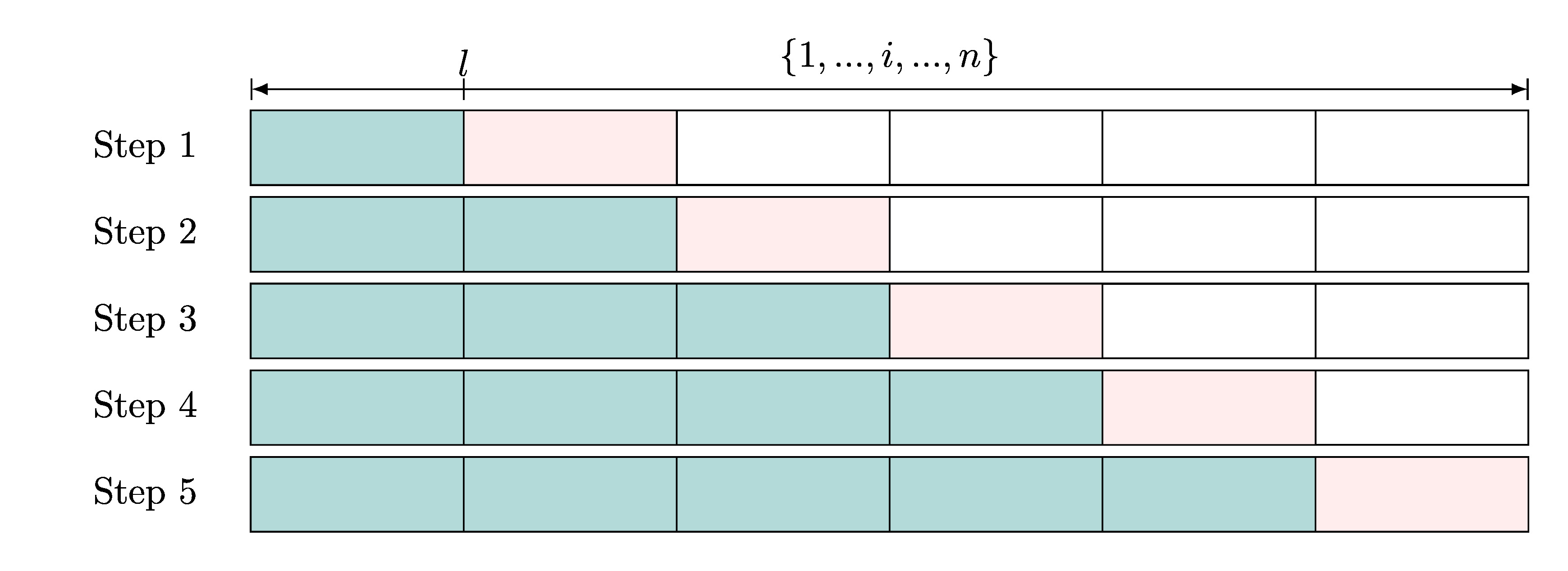
Step 1:

The n observations are randomly ordered. In step 1, the first \{1,...,l\} observations, highlighted in teal/blue, are used to fit the Q-models, g-models, the policy (if using the policy_learn argument), and other required models. We denote the collection of these fitted models as P. The remaining observations are split into M blocks of size m = (n-l)/M, which we for simplicity assume to be a whole number. In step 1, the target parameter is estimated using the associated doubly robust score Z(P) evaluated on the first validation fold highlighted in pink \{l+1,...,l+m\}:

\frac{\sum_{i = l+1}^{l+m} {\widehat \sigma_{i}^{-1}} Z(\widehat P_i)(O_i)} {\sum_{i = l+1}^{l+m} \widehat \sigma_{i}^{-1}},

where \widehat P_i for i \in \{l+1,...,l+m\} refer to the fitted models trained on \{1,...,l\}, and \widehat \sigma_i is the insample estimate for the standard deviation based on the training observations \{1,...,l\}. We will later give an exact expression for \widehat \sigma_i for each target parameter. Note that \widehat \sigma_i is constant for i \in \{l+1,...,l+m\}, but it will be convenient to keep the same index for \widehat \sigma.

Step 2 to M:

In step 2, observations with index \{1,...,l+m\} are used to fit the model collection P, as well as the insample estimate for the standard deviation. For i \in \{l+m+1,...,l+2m\} these are denoted as \widehat P_i, \widehat \sigma_i. This sequential model fitting is repeated for all M steps and the updated online estimator is given by

\frac{\sum_{i = l+1}^{n} {\widehat \sigma_{i}^{-1}} Z(\widehat P_i)(O_i)} {\sum_{i = l+1}^n \widehat \sigma_{i}^{-1}},

with an associated standard error estimate given by

\frac{\left(\frac{1}{n-l}\sum_{i = l+1}^n \widehat \sigma_{i}^{-1}\right)^{-1}}{\sqrt{n-l}}.

Doubly robust scores

target = "value":

For a policy value target the doubly robust score is given by

Z(d, g, Q^d)(O) = Q^d_1(H_1 , d_1(V_1)) + \sum_{r = 1}^K \prod_{j = 1}^{r} \frac{I\{A_j = d_j(\cdot)\}}{g_{j}(H_j, A_j)} \{Q_{r+1}^d(H_{r+1} , d_{r+1}(V_1)) - Q_{r}^d(H_r , d_r(V_1))\}.

The influence function(/curve) for the associated onestep etimator is

Z(d, g, Q^d)(O) - \mathbb{E}[Z(d,g, Q^d)(O)],

which is used to estimate the insample stadard deviation. For example, in step 2, i.e., for i \in \{l+m+1,...,l+2m\}

\widehat \sigma_i^2 = \frac{1}{l+m}\sum_{j=1}^{l+m} \left(Z(\widehat d_i,\widehat Q_i,\widehat{g}_i)(O_j) - \frac{1}{l+m}\sum_{r=1}^{l+m} Z(\widehat d_i,\widehat Q_i,\widehat{g}_i)(O_r) \right)^2

target = "subgroup":

For a subgroup average treatment effect target, where K = 1 (single-stage), \mathcal{A} = \{0,1\} (binary treatment), and d_1(V_1) \in \{s_1, s_2\} (dichotomous subgroup policy) the doubly robust score is given by

Z(d,g,Q, D) = \frac{I\{d_1(\cdot) = s\}}{D} \Big\{Z_1(1,g,Q)(O) - Z_1(0,g,Q)(O) \Big\}.

Z_1(a, g, Q)(O) = Q_1(H_1 , a) + \frac{I\{A = a\}}{g_1(H_1, a)} \{U - Q_{1}(H_1 , a)\},

where D is \mathbb{P}(d_1(V_1) = s).

The associated onestep/estimating equation estimator has influence function

\frac{ I\{d_1(\cdot) = s\}}{D} \Big\{Z_1(1,g,Q)(O) - Z_1(0,g,Q)(O) - E[Z_1(1,g,Q)(O) - Z_1(0,g,Q)(O) | d_1(\cdot) = s]\Big\},

which is used to estimate the standard deviation \widehat \sigma.

Value

policy_eval_online() returns an object of inherited class "policy_eval_online", "policy_eval". The object is a list containing the following elements:

References

Luedtke, Alexander R, and Mark J van der Laan. “STATISTICAL INFERENCE FOR THE MEAN OUTCOME UNDER A POSSIBLY NON-UNIQUE OPTIMAL TREATMENT STRATEGY.” Annals of statistics vol. 44,2 (2016): 713-742. doi:10.1214/15-AOS1384

Create Policy Learner

Description

policy_learn() is used to specify a policy learning method (Q-learning, doubly robust Q-learning, policy tree learning and outcome weighted learning). Evaluating the policy learner returns a policy object.

Usage

policy_learn(
  type = "blip",
  control = control_blip(),
  alpha = 0,
  threshold = NULL,
  full_history = FALSE,
  L = 1,
  cross_fit_g_models = TRUE,
  cross_fit_c_models = TRUE,
  save_cross_fit_models = FALSE,
  future_args = list(future.seed = TRUE),
  name = type
)

## S3 method for class 'policy_learn'
print(x, ...)

## S3 method for class 'policy_object'
print(x, ...)

Arguments

Value

Function of inherited class "policy_learn". Evaluating the function on a policy_data object returns an object of class policy_object. A policy object is a list containing all or some of the following elements:

q_functions

Fitted Q-functions. Object of class "nuisance_functions".

g_functions

Fitted g-functions. Object of class "nuisance_functions".

action_set

Sorted character vector describing the action set, i.e., the possible actions at each stage.

alpha

Numeric. Probability threshold to determine realistic actions.

K

Integer. Maximal number of stages.

qv_functions

(only if type = "drql") Fitted V-restricted Q-functions. Contains a fitted model for each stage and action.

ptl_objects

(only if type = "ptl") Fitted V-restricted policy trees. Contains a policytree::policy_tree for each stage.

ptl_designs

(only if type = "ptl") Specification of the V-restricted design matrix for each stage

S3 generics

The following S3 generic functions are available for an object of class "policy_object":

get_g_functions()

Extract the fitted g-functions.

get_q_functions()

Extract the fitted Q-functions.

get_policy()

Extract the fitted policy object.

get_policy_functions()

Extract the fitted policy function for a given stage.

get_policy_actions()

Extract the (fitted) policy actions.

References

Doubly Robust Q-learning (type = "drql"): Luedtke, Alexander R., and Mark J. van der Laan. "Super-learning of an optimal dynamic treatment rule." The international journal of biostatistics 12.1 (2016): 305-332. doi:10.1515/ijb-2015-0052.

Policy Tree Learning (type = "ptl"): Zhou, Zhengyuan, Susan Athey, and Stefan Wager. "Offline multi-action policy learning: Generalization and optimization." Operations Research (2022). doi:10.1287/opre.2022.2271.

(Augmented) Outcome Weighted Learning: Liu, Ying, et al. "Augmented outcome‐weighted learning for estimating optimal dynamic treatment regimens." Statistics in medicine 37.26 (2018): 3776-3788. doi:10.1002/sim.7844.

See Also

policy_eval()

Examples

library("polle")
### Two stages:
d <- sim_two_stage(5e2, seed=1)
pd <- policy_data(d,
                  action = c("A_1", "A_2"),
                  baseline = c("BB"),
                  covariates = list(L = c("L_1", "L_2"),
                                    C = c("C_1", "C_2")),
                  utility = c("U_1", "U_2", "U_3"))
pd

### V-restricted (Doubly Robust) Q-learning

# specifying the learner:
pl <- policy_learn(
  type = "drql",
  control = control_drql(qv_models = list(q_glm(formula = ~ C_1 + BB),
                                          q_glm(formula = ~ L_1 + BB))),
  full_history = TRUE
)

# evaluating the learned policy
pe <- policy_eval(policy_data = pd,
                  policy_learn = pl,
                  q_models = q_glm(),
                  g_models = g_glm())
pe
# getting the policy object:
po <- get_policy_object(pe)
# inspecting the fitted QV-model for each action strata at stage 1:
po$qv_functions$stage_1
head(get_policy(pe)(pd))

Predict g-functions and Q-functions

Description

predict() returns the fitted values of the g-functions and Q-functions when applied to a (new) policy data object.

Usage

## S3 method for class 'nuisance_functions'
predict(object, new_policy_data, event_set = c(0), ...)

Arguments

Value

data.table::data.table with keys id and stage and variables g_a or Q_a for each action a in the actions set.

Examples

library("polle")
### Single stage:
d <- sim_single_stage(5e2, seed=1)
pd <- policy_data(d, action="A", covariates=list("Z", "B", "L"), utility="U")
pd
# defining a static policy (A=1):
pl <- policy_def(1, name = "A=1")

# doubly robust evaluation of the policy:
pe <- policy_eval(policy_data = pd,
                  policy = pl,
                  g_models = g_glm(),
                  q_models = q_glm())
# summarizing the estimated value of the policy:
pe

# getting the fitted g-function values:
head(predict(get_g_functions(pe), pd))

# getting the fitted Q-function values:
head(predict(get_q_functions(pe), pd))

q_model class object

Description

Use q_glm(), q_glmnet(), q_rf(), and q_sl() to construct an outcome regression model/Q-model object. The constructors are used as input for policy_eval() and policy_learn().

Usage

q_glm(
  formula = ~A * .,
  family = gaussian(),
  model = FALSE,
  na.action = na.pass,
  ...
)

q_glmnet(
  formula = ~A * .,
  family = "gaussian",
  alpha = 1,
  s = "lambda.min",
  ...
)

q_rf(
  formula = ~.,
  num.trees = c(250, 500, 750),
  mtry = NULL,
  cv_args = list(nfolds = 3, rep = 1),
  ...
)

q_sl(
  formula = ~.,
  SL.library = c("SL.mean", "SL.glm"),
  env = parent.frame(),
  onlySL = TRUE,
  discreteSL = FALSE,
  ...
)

q_xgboost(
  formula = ~.,
  objective = "reg:squarederror",
  params = list(),
  nrounds,
  max_depth = 6,
  eta = 0.3,
  nthread = 1,
  cv_args = list(nfolds = 3, rep = 1)
)

Arguments

Details

q_glm() is a wrapper of glm() (generalized linear model).
q_glmnet() is a wrapper of glmnet::glmnet() (generalized linear model via penalized maximum likelihood).
q_rf() is a wrapper of ranger::ranger() (random forest). When multiple hyper-parameters are given, the model with the lowest cross-validation error is selected.
q_sl() is a wrapper of SuperLearner::SuperLearner (ensemble model). q_xgboost() is a wrapper of xgboost::xgboost.

Value

q_model object: function with arguments 'AH' (combined action and history matrix) and 'V_res' (residual value/expected utility).

See Also

get_history_names(), get_q_functions().

Examples

library("polle")
### Single stage case
d1 <- sim_single_stage(5e2, seed=1)
pd1 <- policy_data(d1,
                   action="A",
                   covariates=list("Z", "B", "L"),
                   utility="U")
pd1

# available history variable names for the outcome regression:
get_history_names(pd1)

# evaluating the static policy a=1 using inverse
# propensity weighting based on the given Q-model:
pe1 <- policy_eval(type = "or",
                   policy_data = pd1,
                   policy = policy_def(1, name = "A=1"),
                   q_model = q_glm(formula = ~A*.))
pe1

# getting the fitted Q-function values
head(predict(get_q_functions(pe1), pd1))

### Two stages:
d2 <- sim_two_stage(5e2, seed=1)
pd2 <- policy_data(d2,
                  action = c("A_1", "A_2"),
                  covariates = list(L = c("L_1", "L_2"),
                                    C = c("C_1", "C_2")),
                  utility = c("U_1", "U_2", "U_3"))
pd2

# available full history variable names at each stage:
get_history_names(pd2, stage = 1)
get_history_names(pd2, stage = 2)

# evaluating the static policy a=1 using outcome
# regression based on a glm model for each stage:
pe2 <- policy_eval(type = "or",
            policy_data = pd2,
            policy = policy_def(1, reuse = TRUE, name = "A=1"),
            q_model = list(q_glm(~ A * L_1),
                           q_glm(~ A * (L_1 + L_2))),
            q_full_history = TRUE)
pe2

# getting the fitted Q-function values
head(predict(get_q_functions(pe2), pd2))

Objects exported from other packages

Description

These objects are imported from other packages. Follow the links below to see their documentation.

lava

estimate, IC

SuperLearner

All

Simulate Multi-Stage Data

Description

Simulate Multi-Stage Data

Usage

sim_multi_stage(
  n,
  par = list(tau = 10, gamma = c(0, -0.2, 0.3), alpha = c(0, 0.5, 0.2, -0.5, 0.4), beta =
    c(3, -0.5, -0.5), psi = 1, xi = 0.3),
  a = function(t, x, beta, ...) {
     prob <- lava::expit(beta[1] + (beta[2] * t^2) +
    (beta[3] * x))
     stats::rbinom(n = 1, size = 1, prob = prob)
 },
  seed = NULL
)

Arguments

Details

sim_multi_stage samples n iid observation O with the following distribution:

W \sim \mathcal{N}(0, 1)\\ B \sim Ber(\xi)

For k\geq 1 let

(T_k - T_{k-1})| X_{k-1}, A_{k-1}, W \sim \begin{cases} Exp\Big\{\exp\left(\gamma^T [1, X_{k-1}, W] \right) \Big\} + \psi \quad A_{k-1} = 1\\ \infty \quad A_{k-1} = 0 \end{cases}\\ X_{k}\mid T_k, X_{k-1}, B \sim \begin{cases} \mathcal{N}\left\{ \alpha^T [1, T_k, T^2_k, X_{k-1}, B], 1\right\} \quad T_k < \infty \\ 0 \quad T_k = \infty \end{cases}\\ A_k \mid X_k, T_k \sim \begin{cases} Ber\left\{ expit\left(\beta^T[1, T_{k}^2, X_k] \right)\right\} \quad T_k < \infty\\ 0 \quad T_k = \infty, \end{cases}

Note that \psi is the minimum increment.

Value

list with elements stage_data (data.table::data.table) and baseline_data (data.table::data.table).

Simulate Single-Stage Data

Description

Simulate Single-Stage Data

Usage

sim_single_stage(
  n = 10000,
  par = c(k = 0.1, d = 0.5, a = 1, b = -2.5, c = 3, p = 0.3),
  action_model = function(Z, L, B, k, d) {
     k * (Z + L - 1) * Z^(-2) + d * (B == 1)

    },
  utility_model = function(Z, L, A, a, b, c) {
     Z + L + A * (c * Z + a * L + b)
 },
  seed = NULL,
  return_model = FALSE,
  ...
)

Arguments

Details

sim_single_stage samples n iid observation O = (B, Z, L, A, U) with the following distribution:

B \sim Bernoulli(\pi)\\ Z, L \sim Uniform([0,1])\\ A\mid Z,L,B \sim Bernoulli(expit\{\kappa Z^{-2}(Z+L-1) + \delta B)\\ U\mid Z,L,A \sim \mathcal{N}(Z+L+A\cdot\{\gamma Z + \alpha L + \beta\}, 1)

Value

data.frame with n rows and columns Z, L, B, A, and U.

Simulate Single-Stage Multi-Action Data

Description

Simulate Single-Stage Multi-Action Data

Usage

sim_single_stage_multi_actions(n = 1000, seed = NULL)

Arguments

Details

sim_single_stage_multi_actions samples n iid observation O = (z, x, a, u) with the following distribution:

z, x \sim Uniform([0,1])\\ \tilde a \sim \mathcal{N}(0,1)\\ a \mid \tilde a \sim \begin{cases} 0 \quad if \quad \tilde a < -1\\ 1 \quad if \quad \tilde a -1 \leq a < 0.5\\ 2 \quad otherwise \end{cases}\\ u \mid z, x \sim \mathcal{N}(x + z + I\{a=2\}(x-0.5) + I\{a=1\}(x^2 + z -0.5), 1)

Value

data.frame with n rows and columns z, x, a, and u.

Simulate Two-Stage Data

Description

Simulate Two-Stage Data

Usage

sim_two_stage(
  n = 10000,
  par = c(gamma = 0.5, beta = 1),
  seed = NULL,
  action_model_1 = function(C_1, beta, ...) stats::rbinom(n = NROW(C_1), size = 1, prob =
    lava::expit(beta * C_1)),
  action_model_2 = function(C_2, beta, ...) stats::rbinom(n = NROW(C_2), size = 1, prob =
    lava::expit(beta * C_2)),
  deterministic_rewards = FALSE
)

Arguments

Details

sim_two_stage samples n iid observation O with the following distribution: BB is a random categorical variable with levels group1, group2, and group3. Furthermore,

B \sim \mathcal{N}(0,1)\\ L_{1} \sim \mathcal{N}(0, 1)\\ C_{1} \mid L_{1} \sim \mathcal{N}(L_1, 1)\\ A_1 \mid C_1 \sim Bernoulli(expit(\beta C_1))\\ L_{2} \sim \mathcal{N} (0, 1)\\ C_{2} \mid A_1, L_1 \sim \mathcal{N}(\gamma L_1 + A_1, 1)\\ A_2 \mid C_2 \sim Bernoulli(expit(\beta C_2))\\ L_{3} \sim \mathcal{N} (0, 1)

The rewards are calculated as

U_1 = L_1\\ U_2 = A_1\cdot C_1 + L_2 \\ U_3 = A_2\cdot C_2 + L_3.

Value

data.table::data.table with n rows and columns B, BB, L_1, C_1, A_1, L_2, C_2, A_2, L_3, U_1, U_2, U_3 (,U_1_A0, U_1_A1, U_2_A0, U_2_A1).

Simulate Two-Stage Multi-Action Data

Description

Simulate Two-Stage Multi-Action Data

Usage

sim_two_stage_multi_actions(
  n = 1000,
  par = list(gamma = 0.5, beta = 1, prob = c(0.2, 0.4, 0.4)),
  seed = NULL,
  action_model_1 = function(C_1, beta, ...) stats::rbinom(n = NROW(C_1), size = 1, prob =
    lava::expit(beta * C_1))
)

Arguments

Details

sim_two_stage_multi_actions samples n iid observation O with the following distribution: BB is a random categorical variable with levels group1, group2, and group3. Furthermore,

B \sim \mathcal{N}(0,1)\\ L_{1} \sim \mathcal{N}(0, 1)\\ C_{1} \mid L_{1} \sim \mathcal{N}(L_1, 1)\\ P(A_1='yes'\mid C_1) = expit(\beta C_1)\\ P(A_1='no'\mid C_1) = 1 - P(A_1='yes' \mid C_1)\\ L_{2} \sim \mathcal{N} (0, 1)\\ C_{2} \mid A_1, L_1 \sim \mathcal{N}(\gamma L_1 + A_1, 1)\\ P(A_2='yes') = p_1\\ P(A_2='no') = p_2\\ P(A_2='default') = p_3\\ L_{3} \sim \mathcal{N} (0, 1)

The rewards are calculated as

U_1 = L_1\\ U_2 = A_1\cdot C_1 + L_2 \\ U_3 = A_2\cdot C_2 + L_3.

Value

data.table::data.table with n rows and columns B, BB, L_1, C_1, A_1, L_2, C_2, A_2, L_3, U_1, U_2, U_3.

Subset Policy Data on ID

Description

subset_id returns a policy data object containing the given IDs.

Usage

subset_id(object, id, preserve_action_set = TRUE)

Arguments

Value

Object of class policy_data.

Examples

library("polle")
### Single stage:
d <- sim_single_stage(5e2, seed=1)
# constructing policy_data object:
pd <- policy_data(d, action="A", covariates=list("Z", "B", "L"), utility="U")
pd

# getting the observation IDs:
get_id(pd)[1:10]

# subsetting on IDs:
pdsub <- subset_id(pd, id = 250:500)
pdsub
get_id(pdsub)[1:10]