The hardware and bandwidth for this mirror is donated by dogado GmbH, the Webhosting and Full Service-Cloud Provider. Check out our Wordpress Tutorial.
If you wish to report a bug, or if you are interested in having us mirror your free-software or open-source project, please feel free to contact us at mirror[@]dogado.de.
![]()
![]()
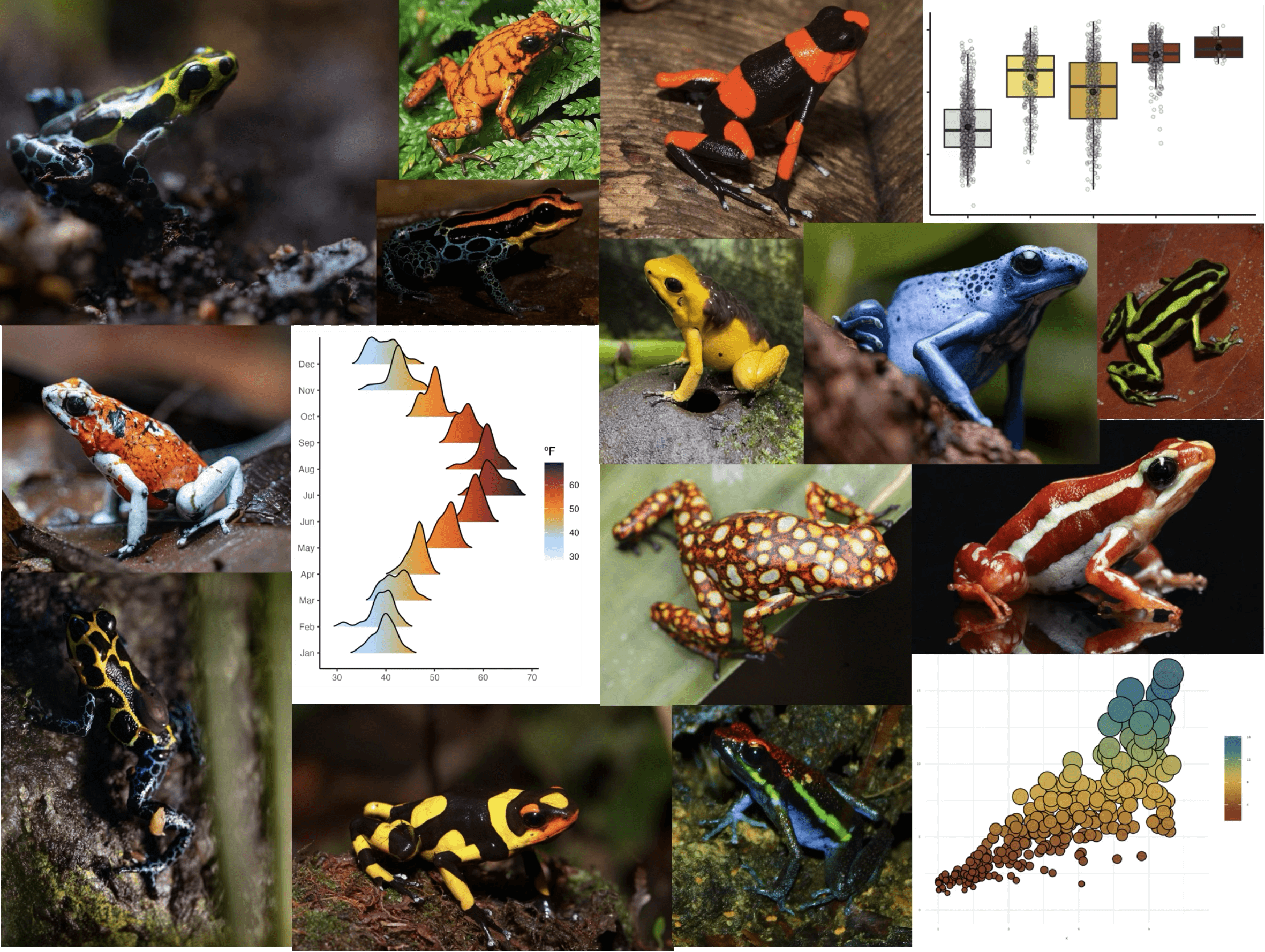
A collection of color palettes inspired by Neotropical poison frogs.
With more than 200 brighly colored species, Neotropical poison frogs
paint the rain forest in vivid hues that shout a clear message: “I’m
toxic!”. Spice up your plots with poisonfrogs and give your
dataviz a toxic twist! But wait, we also included some color palettes
inspired by other pretty frog species, because… why not? 🐸
Get inspired with the collection of species behind the color palettes.
You can install poisonfrogs from CRAN:
install.packages("poisonfrogs")or from the development version in GitHub with:
remotes::install_github("laurenoconnelllab/poisonfrogs")load the package:
library(poisonfrogs)poisonfrogs
color palettes “At a glance”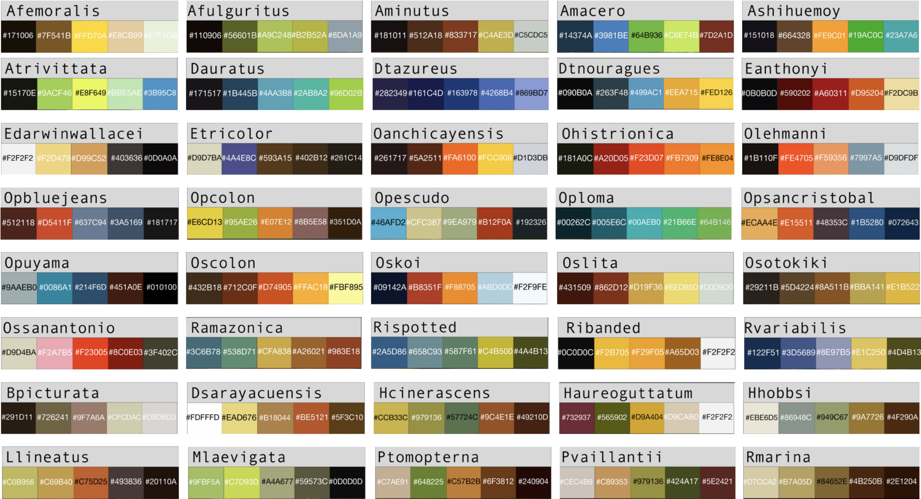
To see the names of all colour palettes in poisonfrogs:
poison_palettes_names()
#>  [1] "Afemoralis"      "Afulguritus"     "Amacero"         "Aminutus"
#>  [5] "Ashihuemoy"      "Atrivittata"     "Bpicturata"      "Dauratus"
#>  [9] "Dsarayacuensis"  "Dtazureus"       "Dtnouragues"     "Eanthonyi"
#> [13] "Edarwinwallacei" "Etricolor"       "Haureoguttatum"  "Hcinerascens"
#> [17] "Hhobbsi"         "Llineatus"       "Mlaevigata"      "Oanchicayensis"
#> [21] "Ohistrionica"    "Olehmanni"       "Opbluejeans"     "Opcolon"
#> [25] "Opescudo"        "Oploma"          "Opsancristobal"  "Opuyama"
#> [29] "Oscolon"         "Oskoi"           "Oslita"          "Osotokiki"
#> [33] "Ossanantonio"    "Pterribilis"     "Ptomopterna"     "Pvaillantii"
#> [37] "Ramazonica"      "Ribanded"        "Rispotted"       "Rmarina"
#> [41] "Rvariabilis"
Visualize poison frog palettes:
poison_palette("Haureoguttatum")
or get their hex codes:
poison_palette("Haureoguttatum", return = "vector")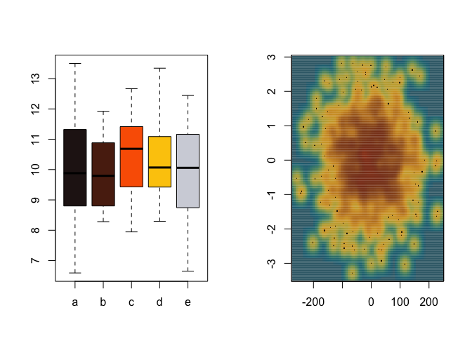
#> [1] "#732937" "#565902" "#D9A404" "#D9CAB0" "#F2F2F2"poisonfrogs in base R plots
par(mfrow = c(1, 2))

#Discrete scale

group <- factor(sample(letters[1:5], 100, replace = TRUE))

value <- rnorm(100, mean = 10, sd = 1.5)

boxplot(value ~ group,
        col = poison_palette(
    "Oanchicayensis",
    return = "vector",
    type = "discrete",
    direction = 1
  ),
  xlab = "",
  ylab = "")

#Continuous scale
x <- rnorm(1000) * 77
y <- rnorm(1000)

smoothScatter(
  y ~ x,
  colramp = colorRampPalette(poison_palette(
    "Ramazonica",
    return = "vector",
    type = "continuous",
    direction = 1
  )),
  xlab = "",
  ylab = ""
)
poison scales in ggplot2scale_fill_poison()
require(tidyverse)
require(gapminder)
require(ggridges)
require(scales)
require(patchwork)

#continuous scale

df_nottem <- tibble(
  year  = floor(time(nottem)),
  month = factor(month.abb[cycle(nottem)], levels = month.abb),
  temp  = as.numeric(nottem)
)

p1 <- ggplot(df_nottem, aes(x = temp, y = month, fill = after_stat(x))) +
  geom_density_ridges_gradient(scale = 2, rel_min_height = 0.01) +
  scale_fill_poison(
    name = "Oskoi",
    type = "continuous",
    alpha = 0.95,
    direction = -1) +
  labs(
  fill = "ºF",
  y = NULL,
  x = NULL) +
  theme_classic(base_size = 10, base_line_size = 0.5) +
  theme(legend.position = "right", legend.justification = "left",
  legend.margin = margin(0,0,0,0),
  legend.box.margin = margin(-5,-5,-5,-5)) +
  coord_cartesian(clip = "off")


#discrete scale
p2 <- ggplot(gapminder, aes(x = continent, y = lifeExp, fill = continent)) +
  geom_boxplot(outliers = F) +
  geom_jitter(
    shape = 21,
    position = position_jitter(0.1),
    alpha = 0.2,
    size = 0.8,
    bg = "grey"
  ) +
  stat_summary(
    fun = mean,
    geom = "point",
    size = 1.5,
    color = "black",
    alpha = 0.6
  ) +
  #theme_classic(base_size = 20, base_line_size = 0.5) +
  scale_fill_poison(
    name = "Amacero",
    type = "discrete",
    alpha = 0.9,
    direction = 1
  ) +
  theme(legend.position = "none") +
  xlab(NULL) +
  ylab("Life Expentancy")

p1 + p2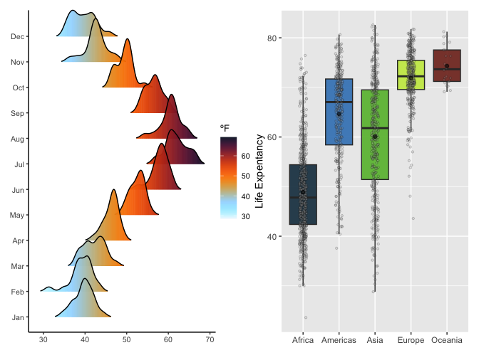
scale_color_poison()
#Continuous scale

set.seed(42)
n <- 300
x <- runif(n, 0, 10)
y <- 1.5 + 0.9 * x + rnorm(n, sd = 0.4 + 0.25 * x)
sz <- rescale(y, to = c(2, 14))

df <- data.frame(x, y, sz)

p3 <- ggplot(df, aes(x, y)) +
  geom_point(
    aes(color = y, size = sz),
    shape = 16,
    alpha = 0.95,
    stroke = 0.6
  ) +
  scale_size_identity(guide = "none") +
  scale_color_poison("Ramazonica", type = "continuous", direction = 1) +
  theme_minimal() +
  ylim(0, 18) +
  xlim(0, 11)


#discrete scale
p4 <- ggplot(gapminder, aes(x = lifeExp, y = log(gdpPercap), colour = continent)) +
  geom_point(alpha = 0.4) +
  scale_colour_poison(name = "Opcolon", type = "discrete") +
  stat_smooth() +
  facet_wrap(.~continent, scales = "free") +
  theme_minimal(10, base_line_size = 0.2) +
  theme(legend.position = "none",
  strip.background = element_blank(), strip.placement = "outside")

p3 + p4 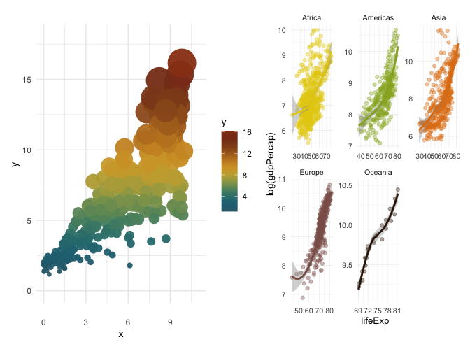
These binaries (installable software) and packages are in development.
They may not be fully stable and should be used with caution. We make no claims about them.
Health stats visible at Monitor.