README

The hardware and bandwidth for this mirror is donated by dogado GmbH, the Webhosting and Full Service-Cloud Provider. Check out our Wordpress Tutorial.
If you wish to report a bug, or if you are interested in having us mirror your free-software or open-source project, please feel free to contact us at mirror[@]dogado.de.

pminternal: Internal Validation of Clinical Prediction Models

The goal is to offer a package that can produce bias-corrected performance measures for clinical prediction models with binary outcomes for a range of model development approaches available in R (similar to rms::validate). There are also functions for assessing prediction stability, as described in Riley and Collins (2023).

install.packages("pminternal") # cran
# or 
devtools::install_github("stephenrho/pminternal") # development

Example

In the example below we use bootstrapping to correct performance measures for a glm via calculation of ‘optimism’ (see vignette("pminternal"), vignette("validate-examples"), and vignette("missing-data") for more examples):

library(pminternal)

# make some data
set.seed(2345)
n <- 800
p <- 10

X <- matrix(rnorm(n*p), nrow = n, ncol = p)
LP <- -1 + apply(X[, 1:5], 1, sum) # first 5 variables predict outcome
y <- rbinom(n, 1, plogis(LP))

dat <- data.frame(y, X)

# fit a model
mod <- glm(y ~ ., data = dat, family = "binomial")

# calculate bootstrap optimism corrected performance measures
(val <- validate(fit = mod, method = "boot_optimism", B = 100))
#> It is recommended that B >= 200 for bootstrap validation
#>           apparent optimism corrected   n
#> C           0.8567   0.0093    0.8474 100
#> Brier       0.1423  -0.0054    0.1477 100
#> Intercept   0.0000   0.0175   -0.0175 100
#> Slope       1.0000   0.0529    0.9471 100
#> Eavg        0.0045  -0.0048    0.0093 100
#> E50         0.0039  -0.0050    0.0089 100
#> E90         0.0081  -0.0107    0.0187 100
#> Emax        0.0109  -0.0057    0.0165 100
#> ECI         0.0027  -0.0038    0.0065 100

The other available methods for calculating bias corrected performance are the simple bootstrap (boot_simple), 0.632 bootstrap optimism (.632), optimism via cross-validation (cv_optimism), and regular cross-validation (cv_average). Please see ?pminternal::validate and the references therein. Bias corrected calibration curves can also be produced (see pminternal::cal_plot). Confidence intervals can also be added via confint.

For models that cannot be supported via fit, users are able to specify their own model (model_fun) and prediction (pred_fun) functions as shown below. Note that when specifying user-defined model and prediction functions the data and outcome must also be provided. It is crucial that model_fun implements the entire model development procedure (variable selection, hyperparameter tuning, etc). For more examples, see vignette("pminternal") and vignette("validate-examples").

# fit a glm with lasso penalty
library(glmnet)
#> Loading required package: Matrix
#> Loaded glmnet 4.1-8

lasso_fun <- function(data, ...){
  y <- data$y
  x <- as.matrix(data[, which(colnames(data) != "y")])
  
  cv <- cv.glmnet(x=x, y=y, alpha=1, nfolds = 10, family="binomial")
  lambda <- cv$lambda.min
  
  glmnet(x=x, y=y, alpha = 1, lambda = lambda, family="binomial")
}

lasso_predict <- function(model, data, ...){
  y <- data$y
  x <- as.matrix(data[, which(colnames(data) != "y")])
  
  predict(model, newx = x, type = "response")[,1]
}

(val <- validate(data = dat, outcome = "y", 
                 model_fun = lasso_fun, pred_fun = lasso_predict, 
                 method = "boot_optimism", B = 100))
#> It is recommended that B >= 200 for bootstrap validation
#>           apparent optimism corrected   n
#> C            0.856   0.0070     0.849 100
#> Brier        0.143  -0.0041     0.147 100
#> Intercept    0.080   0.0191     0.061 100
#> Slope        1.155   0.0449     1.110 100
#> Eavg         0.020   0.0013     0.019 100
#> E50          0.019   0.0026     0.017 100
#> E90          0.040   0.0021     0.038 100
#> Emax         0.044   0.0145     0.029 100
#> ECI          0.053   0.0087     0.044 100

The output of validate (with method = "boot_*") can be used to produce plots for assessing the stability of model predictions (across models developed on bootstrap resamples).

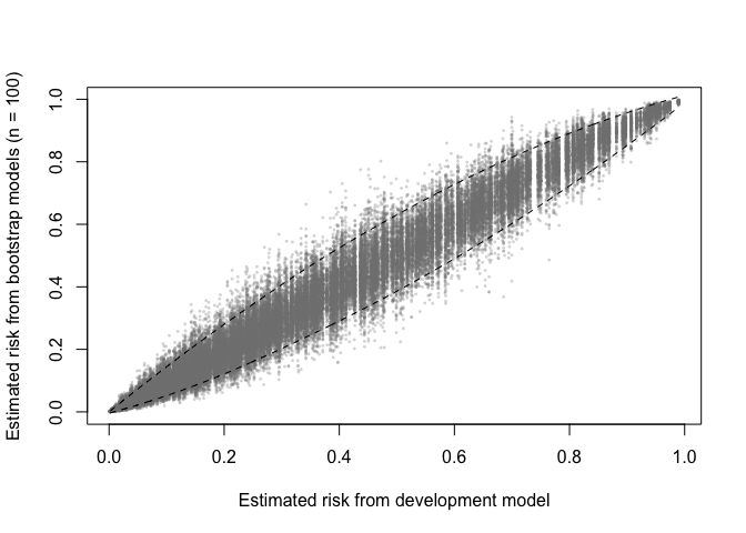
A prediction (in)stability plot shows predictions from the B (in this case 100) bootstrap models applied to the development data.

prediction_stability(val, smooth_bounds = TRUE)

A MAPE plot shows the mean absolute prediction error, which is the difference between the predicted risk from the development model and each of the B bootstrap models.

mape_stability(val)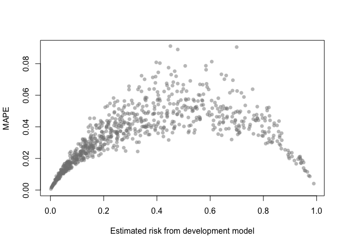

A calibration (in)stability plot depict the original calibration curve along with B calibration curves from the bootstrap models applied to the original data (y).

calibration_stability(val)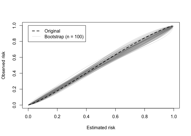

The classification instability index (CII) is the proportion of individuals that change predicted class (present/absent, 1/0) when predicted risk is compared to some threshold. For example, a patient predicted to be in class 1 would receive a CII of 0.3 if 30% of the bootstrap models led to a predicted class of 0.

classification_stability(val, threshold = .4)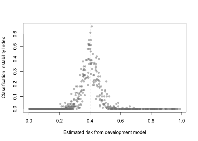

Decision curves implied by the original and bootstrap models can also be plotted.

dcurve_stability(val)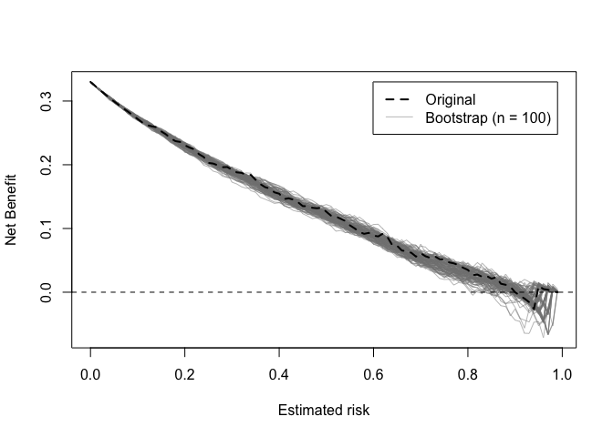

These binaries (installable software) and packages are in development.
They may not be fully stable and should be used with caution. We make no claims about them.
Health stats visible at Monitor.