The hardware and bandwidth for this mirror is donated by dogado GmbH, the Webhosting and Full Service-Cloud Provider. Check out our Wordpress Tutorial.
If you wish to report a bug, or if you are interested in having us mirror your free-software or open-source project, please feel free to contact us at mirror[@]dogado.de.
![]()
![]()
![]()
install.packages("overtureR")

# devtools::install_github("arthurgailes/overtureR")dplyr and sf integrationsf data within
duckdb or with sfReplicating duckdb examples fromm the Overture
docs
library(overtureR)
library(dplyr)
library(ggplot2)
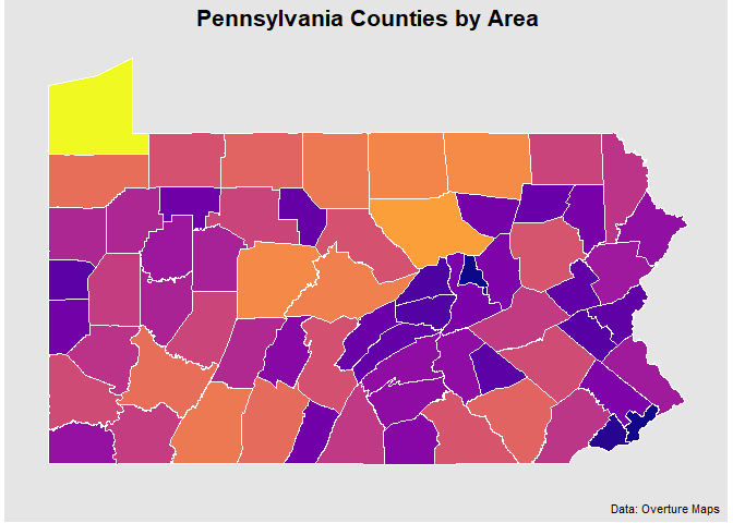
counties <- open_curtain("division_area") |>
# in R, filtering on variables must come before removing them via select
filter(subtype == "county" & country == "US" & region == "US-PA") |>
transmute(
id,
division_id,
primary = names$primary,
geometry
) |>
collect()
# Plot the results
ggplot(counties) +
geom_sf(aes(fill = as.numeric(sf::st_area(geometry))), color = "white", size = 0.2) +
viridis::scale_fill_viridis(option = "plasma", guide = FALSE) +
labs(
title = "Pennsylvania Counties by Area",
caption = "Data: Overture Maps"
) 
library(overtureR)
library(dplyr)

# lazily load the full `mountains` dataset
mountains <- open_curtain(type = "*", theme = "places") |>
  transmute(
    id,
    primary_name = names$primary,
    x = bbox$xmin,
    y = bbox$ymin,
    main_category = categories$primary,
    primary_source = sources[[1]]$dataset,
    confidence,
    geometry # currently no duckdb spatial implementation
  ) |>
  filter(main_category == "mountain" & confidence > .90)

head(mountains)
#> # Source:   SQL [6 x 8]
#> # Database: DuckDB v1.0.0 [Arthur.Gailes@Windows 10 x64:R 4.2.1/:memory:]
#>   id            primary_name     x     y main_category primary_source confidence
#>   <chr>         <chr>        <dbl> <dbl> <chr>         <chr>               <dbl>
#> 1 08f464e0e312… Kawaikini    -159.  22.1 mountain      meta                0.954
#> 2 08f464e3b1a2… Kalepa       -159.  22.0 mountain      meta                0.938
#> 3 08f464e05984… Sleeping Gi… -159.  22.1 mountain      meta                0.945
#> 4 08f464e3a4d0… Nounou-East… -159.  22.1 mountain      meta                0.945
#> 5 08f464e05514… Makaleha Mo… -159.  22.1 mountain      meta                0.965
#> 6 08f464e03538… Makana       -160.  22.2 mountain      meta                0.938
#> # ℹ 1 more variable: geometry <POINT [°]>The record_overture function allows you to download Overture Maps data to a local directory, maintaining the same partition structure as in S3. This is useful for offline analysis or when you need to work with the data repeatedly. Here’s an example:
library(overtureR)
library(ggplot2)
library(dplyr)
library(rayshader)

# Define a bounding box for New York City
broadway <- c(xmin = -73.9901, ymin = 40.755488, xmax = -73.98, ymax = 40.76206)

# Download building data for NYC to a local directory
local_buildings <- open_curtain("building", broadway) |>
  record_overture(output_dir = tempdir(), overwrite = TRUE)

# The downloaded data is returned as a `dbplyr` object, same as the original (but faster!)
broadway_buildings <- local_buildings |>
  filter(!is.na(height)) |>
  mutate(height = round(height)) |>
  collect()

p <- ggplot(broadway_buildings) +
  geom_sf(aes(fill = height)) +
  scale_fill_distiller(palette = "Oranges", direction = 1) +
  # guides(fill = FALSE) +
  labs(title = "Buildings on Broadway", caption = "Data: Overture Maps", fill = "")

# Convert to 3D and render
plot_gg(
  p,
  multicore = TRUE,
  width = 6, height = 5, scale = 250,
  windowsize = c(1032, 860),
  zoom = 0.55,
  phi = 40, theta = 0,
  solid = FALSE,
  offset_edges = TRUE,
  sunangle = 75
)

render_snapshot(clear=TRUE)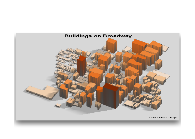
These binaries (installable software) and packages are in development.
They may not be fully stable and should be used with caution. We make no claims about them.
Health stats visible at Monitor.