The hardware and bandwidth for this mirror is donated by dogado GmbH, the Webhosting and Full Service-Cloud Provider. Check out our Wordpress Tutorial.
If you wish to report a bug, or if you are interested in having us mirror your free-software or open-source project, please feel free to contact us at mirror[@]dogado.de.
![]()
outlierensembles provides a collection of outlier/anomaly detection ensembles. Given the anomaly scores of different anomaly detection methods, the following ensemble techniques can be used to construct an ensemble score:
You can install the released version of outlierensembles from CRAN with:
install.packages("outlierensembles")And the development version from GitHub with:
# install.packages("devtools")
devtools::install_github("sevvandi/outlierensembles")
Then load the libraries.
library(outlierensembles)
library(ggplot2)We use methods from dbscan R package as to find anomalies. You can use any anomaly detection method you want to build the ensemble. First, we construct the IRT ensemble. The colors show the ensemble scores.
faithfulu <- scale(faithful)
if (requireNamespace("dbscan", quietly = TRUE)){

  # Using different parameters of lof for anomaly detection
  y1 <- dbscan::lof(faithfulu, minPts = 5)
  y2 <- dbscan::lof(faithfulu, minPts = 10)
  y3 <- dbscan::lof(faithfulu, minPts = 20)
  knnobj <- dbscan::kNN(faithfulu, k = 20)
  # Using different KNN distances as anomaly scores
  y4 <- knnobj$dist[ ,5]
  y5 <- knnobj$dist[ ,10]
  y6 <- knnobj$dist[ ,20]
  # Dense points are less anomalous. Points in less dense areas are more anomalous. Hence 1 - pointdensity is used.
  y7 <- 1 - dbscan::pointdensity(faithfulu, eps = 1, type="gaussian")
  y8 <- 1 - dbscan::pointdensity(faithfulu, eps = 2, type = "gaussian")
  y9 <- 1 - dbscan::pointdensity(faithfulu, eps = 0.5, type = "gaussian")

  Yfaithful <- cbind.data.frame(y1, y2, y3, y4, y5, y6, y7, y8, y9)

}else{
  # If dbscan is not installed, then load data from package
  data(Yfaithful)
}

Y <- Yfaithful
ens1 <- irt_ensemble(Y)
#> Warning in sqrt(diag(solve(Hess))): NaNs produced
df <- cbind.data.frame(faithful, ens1$scores)
colnames(df)[3] <- "IRT"
ggplot(df, aes(eruptions, waiting)) + geom_point(aes(color=IRT)) + scale_color_gradient(low="yellow", high="red") 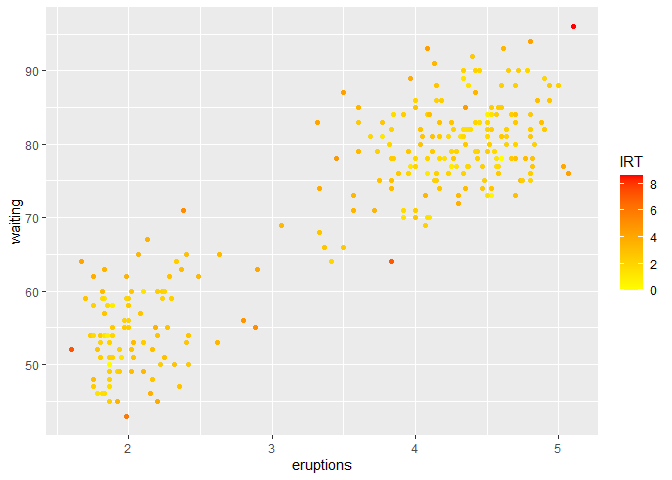
Then we do the greedy ensemble.
ens2 <- greedy_ensemble(Y)
df <- cbind.data.frame(faithful, ens2$scores)
colnames(df)[3] <- "Greedy"
ggplot(df, aes(eruptions, waiting)) + geom_point(aes(color=Greedy)) + scale_color_gradient(low="yellow", high="red") 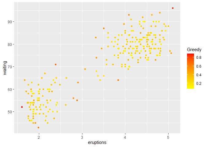
We do the ICWA ensemble next.
ens3 <- icwa_ensemble(Y)
df <- cbind.data.frame(faithful, ens3)
colnames(df)[3] <- "ICWA"
ggplot(df, aes(eruptions, waiting)) + geom_point(aes(color=ICWA)) + scale_color_gradient(low="yellow", high="red") 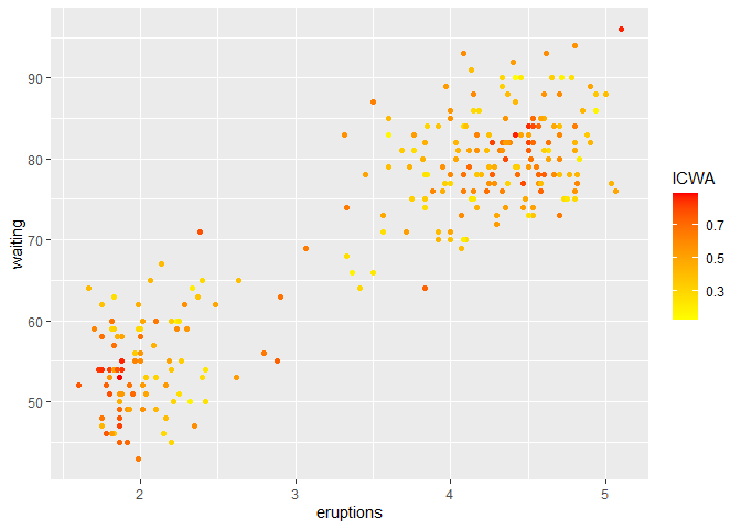
Next, we use the maximum scores to build the ensemble.
ens4 <- max_ensemble(Y)
df <- cbind.data.frame(faithful, ens4)
colnames(df)[3] <- "Max"
ggplot(df, aes(eruptions, waiting)) + geom_point(aes(color=Max)) + scale_color_gradient(low="yellow", high="red") 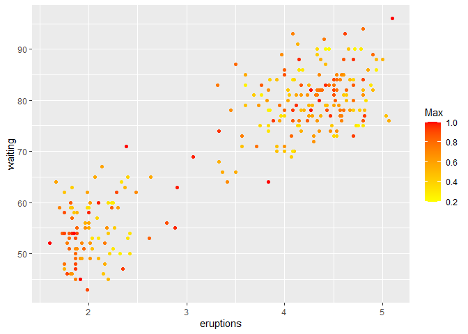
Then, we use the a threshold sum to construct the ensemble.
ens5 <- threshold_ensemble(Y)
df <- cbind.data.frame(faithful, ens5)
colnames(df)[3] <- "Threshold"
ggplot(df, aes(eruptions, waiting)) + geom_point(aes(color=Threshold)) + scale_color_gradient(low="yellow", high="red") 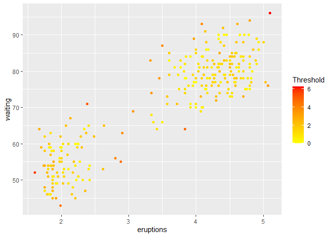
Finally, we use the mean values as the ensemble score.
ens6 <- average_ensemble(Y)
df <- cbind.data.frame(faithful, ens6)
colnames(df)[3] <- "Average"
ggplot(df, aes(eruptions, waiting)) + geom_point(aes(color=Average)) + scale_color_gradient(low="yellow", high="red") 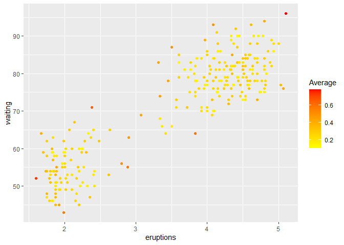
These binaries (installable software) and packages are in development.
They may not be fully stable and should be used with caution. We make no claims about them.
Health stats visible at Monitor.