The hardware and bandwidth for this mirror is donated by dogado GmbH, the Webhosting and Full Service-Cloud Provider. Check out our Wordpress Tutorial.
If you wish to report a bug, or if you are interested in having us mirror your free-software or open-source project, please feel free to contact us at mirror[@]dogado.de.

osfr

Overview

osfr provides a suite of functions for interacting with the Open Science Framework (OSF).

What is OSF?

OSF is a free and open source project management repository designed to support researchers across their entire project lifecycle. The service includes unlimited cloud storage and file version history, providing a centralized location for all your research materials that can be kept private, shared with select collaborators, or made publicly available with citable DOIs.

Installation

You can install the current release of osfr from CRAN (recommended):

install.packages("osfr")

Or the development version from GitHub with the remotes package:

# install.packages("remotes")
remotes::install_github("ropensci/osfr")

Usage Examples

Note: You need to setup an OSF personal access token (PAT) to use osfr to manage projects or upload files.

Accessing Open Research Materials

Many researchers use OSF to archive and share their work. You can use osfr to explore publicly accessible projects and download the associated files—all you need to get started is the project’s URL or GUID (global unique identifier).

Every user, project, component, and file on OSF is assigned a GUID that is embedded in the corresponding entity’s URL. For example, you can access the main OSF project for the Cancer Reproducibility Project at https://osf.io/e81xl/. The GUID for this project is e81xl.

We can then use osfr to retrieve this project and load it into R by providing the GUID:

library(osfr)

cr_project <- osf_retrieve_node("e81xl")
cr_project
#> # A tibble: 1 × 3
#>   name                                    id    meta            
#>   <chr>                                   <chr> <list>          
#> 1 Reproducibility Project: Cancer Biology e81xl <named list [3]>

This returns an osf_tbl object with a single row representing the retrieved project. Let’s list the files that have been uploaded to this project.

osf_ls_files(cr_project)
#> # A tibble: 4 × 3
#>   name                                        id                    meta        
#>   <chr>                                       <chr>                 <list>      
#> 1 papers_and_keywords.xlsx                    553e671b8c5e4a219919… <named list>
#> 2 Full_dataset_of_papers_formatted.xls        553e671b8c5e4a219919… <named list>
#> 3 METHOD_to_select_papers.txt                 553e671b8c5e4a219919… <named list>
#> 4 Adjustment of 50 studies to 37 studies.docx 565602398c5e4a3877d7… <named list>

This returns another osf_tbl with 1 row for each of the files and directories in the project. We can examine any of these files directly on OSF with osf_open(), which opens the corresponding file’s view in your default browser.

This project contains 2 components: Replication Studies and Data collection and publishing guidelines. We can list these components with osfr using osf_ls_nodes().

osf_ls_nodes(cr_project)
#> # A tibble: 5 × 3
#>   name                                                        id    meta        
#>   <chr>                                                       <chr> <list>      
#> 1 Meta-analysis paper figures and tables                      squy7 <named list>
#> 2 Replication Data from the Reproducibility Project: Cancer … e5nvr <named list>
#> 3 Process paper figures and reported statistics               35ut8 <named list>
#> 4 Replication Studies                                         p7ayb <named list>
#> 5 Data collection and publishing guidelines                   a5imq <named list>

osfr is compatible with the pipe operator and dplyr, providing a powerful set of tools for working with osf_tbls. Here, we’re listing the sub-components nested within the Replication Studies component, filtering for a specific study (Study 19) and then listing the files uploaded to that study’s component.

library(dplyr)

cr_project %>%
  osf_ls_nodes() %>%
  filter(name == "Replication Studies") %>%
  osf_ls_nodes(pattern = "Study 19") %>%
  osf_ls_files()
#> # A tibble: 6 × 3
#>   name                                      id                      meta        
#>   <chr>                                     <chr>                   <list>      
#> 1 Replication_Study_19.Rmd                  578e2b23594d9001f48164… <named list>
#> 2 Study_19_Correction_Letter.docx           5a56569125719b000ff28b… <named list>
#> 3 Replication_Study_19.docx                 57c9e8ed594d9001e7a240… <named list>
#> 4 Response_letter_Replication_Study_19.docx 58755747b83f6901ff066a… <named list>
#> 5 Replication_Study_19_track_changes.docx   581a27b76c613b02233228… <named list>
#> 6 Replication_Study_19_track_changes_2.docx 58714d46594d9001f801f4… <named list>

We could continue this pattern of exploration and even download local copies of project files using osf_download(). Or, if you come across a publication that directly references a file’s OSF URL, you could quickly download it to your project directory by providing the URL or simply the GUID:

osf_retrieve_file("https://osf.io/btgx3/") %>%
  osf_download()
#> # A tibble: 1 × 4
#>   name                  id    local_path              meta            
#>   <chr>                 <chr> <chr>                   <list>          
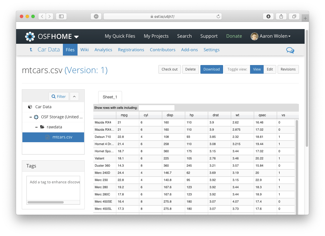
#> 1 Study_19_Figure_1.pdf btgx3 ./Study_19_Figure_1.pdf <named list [3]>

Managing Projects

You can use osfr to create projects, add sub-components or directories, and upload files. See Getting Started to learn more about building projects with osfr, but here is a quick example in which we:

1. Create a new project called Motor Trend Car Road Tests
2. Create a sub-component called Car Data
3. Create a directory named rawdata
4. Upload a file (mtcars.csv) to the new directory
5. Open the uploaded file on OSF

# create an external data file
write.csv(mtcars, "mtcars.csv")

osf_create_project(title = "Motor Trend Car Road Tests") %>%
  osf_create_component("Car Data") %>%
  osf_mkdir("rawdata") %>%
  osf_upload("mtcars.csv") %>%
  osf_open()

Details on osf_tbls

There are 3 main types of OSF entities that osfr can work with:

1. nodes: both projects and components (i.e., sub-projects) are referred to as nodes
2. files: this includes both files and folders stored on OSF
3. users: individuals with OSF accounts

osfr represents these entities within osf_tbls—specialized data frames built on the tibble class that provide useful information about the entities like their name and unique id for users, and API data in the meta column that’s necessary for osfr’s internal functions. Otherwise, they’re just data.frames and can be manipulated using standard functions from base R or dplyr.

Acknowledgments

OSF is developed by the Center for Open Science in Charlottesville, VA.

The original version of osfr was developed by Chris Chartgerink and further developed by Brian Richards and Ryan Hafen. The current version was developed by Aaron Wolen and is heavily inspired by Jennifer Bryan and Lucy D’Agostino McGowan’s excellent googledrive package. Seriously, we borrowed a lot of great ideas from them. Other important resources include http testing by Scott Chamberlain and R Packages by Hadley Wickham. Development was also greatly facilitated by OSF’s excellent API documentation.

Big thanks to Rusty Speidel for designing our logo and Tim Errington for his feedback during development.

Contributing

Check out the Contributing Guidelines to get started with osfr development and note that by contributing to this project, you agree to abide by the terms outlined in the Contributor Code of Conduct.

These binaries (installable software) and packages are in development.
They may not be fully stable and should be used with caution. We make no claims about them.
Health stats visible at Monitor.