The hardware and bandwidth for this mirror is donated by dogado GmbH, the Webhosting and Full Service-Cloud Provider. Check out our Wordpress Tutorial.
If you wish to report a bug, or if you are interested in having us mirror your free-software or open-source project, please feel free to contact us at mirror[@]dogado.de.
The oem package provides estimation for various penalized linear models using the Orthogonalizing EM algorithm. Documentation for the package can be found here: oem site.
Install using the devtools package (RcppEigen must be installed first as well):
devtools::install_github("jaredhuling/oem")or by cloning and building using R CMD INSTALL
To cite oem please use:
Xiong, S., Dai, B., Huling, J., Qian, P. Z. G. (2016) Orthogonalizing
EM: A design-based least squares algorithm, Technometrics, Volume 58,
Pages 285-293,
http://dx.doi.org/10.1080/00401706.2015.1054436.
Huling, J.D. and Chien, P. (2018), Fast Penalized Regression and Cross Validation for Tall Data with the OEM Package, Journal of Statistical Software, to appear, URL: https://arxiv.org/abs/1801.09661.
library(microbenchmark)
library(glmnet)
library(oem)
# compute the full solution path, n > p
set.seed(123)
n <- 1000000
p <- 100
m <- 25
b <- matrix(c(runif(m), rep(0, p - m)))
x <- matrix(rnorm(n * p, sd = 3), n, p)
y <- drop(x %*% b) + rnorm(n)

lambdas = oem(x, y, intercept = TRUE, standardize = FALSE, penalty = "elastic.net")$lambda[[1]]

microbenchmark(
    "glmnet[lasso]" = {res1 <- glmnet(x, y, thresh = 1e-10,
                                      standardize = FALSE,
                                      intercept = TRUE,
                                      lambda = lambdas)},
    "oem[lasso]"    = {res2 <- oem(x, y,
                                   penalty = "elastic.net",
                                   intercept = TRUE,
                                   standardize = FALSE,
                                   lambda = lambdas,
                                   tol = 1e-10)},
    times = 5
)
## Unit: seconds
## expr min lq mean median uq max neval cld
## glmnet[lasso] 5.325385 5.374823 5.859432 6.000302 6.292411 6.304239 5 a
## oem[lasso] 1.539320 1.573569 1.600241 1.617136 1.631450 1.639730 5 b# difference of results
max(abs(coef(res1) - res2$beta[[1]]))## [1] 1.048243e-07res1 <- glmnet(x, y, thresh = 1e-12,
standardize = FALSE,
intercept = TRUE,
lambda = lambdas)
# answers are now more close once we require more precise glmnet solutions
max(abs(coef(res1) - res2$beta[[1]]))## [1] 3.763507e-09library(sparsenet)
library(ncvreg)
# compute the full solution path, n > p
set.seed(123)
n <- 5000
p <- 200
m <- 25
b <- matrix(c(runif(m, -0.5, 0.5), rep(0, p - m)))
x <- matrix(rnorm(n * p, sd = 3), n, p)
y <- drop(x %*% b) + rnorm(n)
mcp.lam <- oem(x, y, penalty = "mcp",
gamma = 2, intercept = TRUE,
standardize = TRUE,
nlambda = 200, tol = 1e-10)$lambda[[1]]
scad.lam <- oem(x, y, penalty = "scad",
gamma = 4, intercept = TRUE,
standardize = TRUE,
nlambda = 200, tol = 1e-10)$lambda[[1]]
microbenchmark(
"sparsenet[mcp]" = {res1 <- sparsenet(x, y, thresh = 1e-10,
gamma = c(2,3), #sparsenet throws an error
#if you only fit 1 value of gamma
nlambda = 200)},
"oem[mcp]" = {res2 <- oem(x, y,
penalty = "mcp",
gamma = 2,
intercept = TRUE,
standardize = TRUE,
nlambda = 200,
tol = 1e-10)},
"ncvreg[mcp]" = {res3 <- ncvreg(x, y,
penalty = "MCP",
gamma = 2,
lambda = mcp.lam,
eps = 1e-7)},
"oem[scad]" = {res4 <- oem(x, y,
penalty = "scad",
gamma = 4,
intercept = TRUE,
standardize = TRUE,
nlambda = 200,
tol = 1e-10)},
"ncvreg[scad]" = {res5 <- ncvreg(x, y,
penalty = "SCAD",
gamma = 4,
lambda = scad.lam,
eps = 1e-7)},
times = 5
)## Unit: milliseconds
## expr min lq mean median uq
## sparsenet[mcp] 1466.54465 1492.72548 1527.32113 1517.19926 1579.70827
## oem[mcp] 95.71381 98.09740 105.90083 105.76415 110.31668
## ncvreg[mcp] 5196.48035 5541.69429 5669.10010 5611.31491 5865.06723
## oem[scad] 70.74110 71.46554 80.21926 78.76494 84.25458
## ncvreg[scad] 5289.59790 5810.69254 5801.60997 5950.84377 5964.01276
## max neval cld
## 1580.42800 5 a
## 119.61209 5 b
## 6130.94372 5 c
## 95.87013 5 b
## 5992.90288 5 cdiffs <- array(NA, dim = c(2, 1))
colnames(diffs) <- "abs diff"
rownames(diffs) <- c("MCP: oem and ncvreg", "SCAD: oem and ncvreg")
diffs[,1] <- c(max(abs(res2$beta[[1]] - res3$beta)), max(abs(res4$beta[[1]] - res5$beta)))
diffs## abs diff
## MCP: oem and ncvreg 1.725859e-07
## SCAD: oem and ncvreg 5.094648e-08In addition to the group lasso, the oem package offers computation for the group MCP, group SCAD, and group sparse lasso penalties. All aforementioned penalties can also be augmented with a ridge penalty.
library(gglasso)
library(grpreg)
library(grplasso)
# compute the full solution path, n > p
set.seed(123)
n <- 10000
p <- 200
m <- 25
b <- matrix(c(runif(m, -0.5, 0.5), rep(0, p - m)))
x <- matrix(rnorm(n * p, sd = 3), n, p)
y <- drop(x %*% b) + rnorm(n)
groups <- rep(1:floor(p/10), each = 10)

grp.lam <- oem(x, y, penalty = "grp.lasso",
               groups = groups,
               nlambda = 100, tol = 1e-10)$lambda[[1]]


microbenchmark(
    "gglasso[grp.lasso]" = {res1 <- gglasso(x, y, group = groups,
                                            lambda = grp.lam,
                                            intercept = FALSE,
                                            eps = 1e-8)},
    "oem[grp.lasso]"    = {res2 <- oem(x, y,
                                       groups = groups,
                                       intercept = FALSE,
                                       standardize = FALSE,
                                       penalty = "grp.lasso",
                                       lambda = grp.lam,
                                       tol = 1e-10)},
    "grplasso[grp.lasso]"    = {res3 <- grplasso(x=x, y=y,
                                                 index = groups,
                                                 standardize = FALSE,
                                                 center = FALSE, model = LinReg(),
                                                 lambda = grp.lam * n * 2,
                                                 control = grpl.control(trace = 0, tol = 1e-10))},
    "grpreg[grp.lasso]"    = {res4 <- grpreg(x, y, group = groups,
                                             eps = 1e-10, lambda = grp.lam)},
    times = 5
)
## Unit: milliseconds
## expr min lq mean median uq
## gglasso[grp.lasso] 679.59049 724.16350 858.99280 801.79179 865.83580
## oem[grp.lasso] 59.84769 62.23879 64.11779 63.36026 64.30146
## grplasso[grp.lasso] 3714.92601 3753.18663 4322.32431 4537.50185 4786.80867
## grpreg[grp.lasso] 1216.21794 1248.84647 1270.46132 1269.71047 1287.75969
## max neval cld
## 1223.58241 5 a
## 70.84075 5 b
## 4819.19839 5 c
## 1329.77201 5 adiffs <- array(NA, dim = c(2, 1))
colnames(diffs) <- "abs diff"
rownames(diffs) <- c("oem and gglasso", "oem and grplasso")
diffs[,1] <- c( max(abs(res2$beta[[1]][-1,] - res1$beta)), max(abs(res2$beta[[1]][-1,] - res3$coefficients)) )
diffs## abs diff
## oem and gglasso 1.303906e-06
## oem and grplasso 1.645871e-08set.seed(123)
n <- 500000
p <- 200
m <- 25
b <- matrix(c(runif(m, -0.5, 0.5), rep(0, p - m)))
x <- matrix(rnorm(n * p, sd = 3), n, p)
y <- drop(x %*% b) + rnorm(n)
groups <- rep(1:floor(p/10), each = 10)
# fit all group penalties at once
grp.penalties <- c("grp.lasso", "grp.mcp", "grp.scad",
"grp.mcp.net", "grp.scad.net",
"sparse.group.lasso")
system.time(res <- oem(x, y,
penalty = grp.penalties,
groups = groups,
alpha = 0.25, # mixing param for l2 penalties
tau = 0.5)) # mixing param for sparse grp lasso ## user system elapsed
## 2.043 0.222 2.267The oem algorithm is quite efficient at fitting multiple penalties simultaneously when p is not too big.
set.seed(123)
n <- 100000
p <- 100
m <- 15
b <- matrix(c(runif(m, -0.25, 0.25), rep(0, p - m)))
x <- matrix(rnorm(n * p, sd = 3), n, p)
y <- drop(x %*% b) + rnorm(n)

microbenchmark(
    "oem[lasso]"    = {res1 <- oem(x, y,
                                   penalty = "elastic.net",
                                   intercept = TRUE,
                                   standardize = TRUE,
                                   tol = 1e-10)},
    "oem[lasso/mcp/scad/ols]"    = {res2 <- oem(x, y,
                                   penalty = c("elastic.net", "mcp",
                                               "scad", "grp.lasso",
                                               "grp.mcp", "sparse.grp.lasso",
                                               "grp.mcp.net", "mcp.net"),
                                   gamma = 4,
                                   tau = 0.5,
                                   alpha = 0.25,
                                   groups = rep(1:10, each = 10),
                                   intercept = TRUE,
                                   standardize = TRUE,
                                   tol = 1e-10)},
    times = 5
)
## Unit: milliseconds
## expr min lq mean median uq max
## oem[lasso] 125.6408 126.7870 130.3534 127.3374 133.4962 138.5055
## oem[lasso/mcp/scad/ols] 148.3162 152.1743 153.0176 152.4529 154.4300 157.7144
## neval cld
## 5 a
## 5 b#png("../mcp_path.png", width = 3000, height = 3000, res = 400);par(mar=c(5.1,5.1,4.1,2.1));plot(res2, which.model = 2, main = "mcp",lwd = 3,cex.axis=2.0, cex.lab=2.0, cex.main=2.0, cex.sub=2.0);dev.off()
#
layout(matrix(1:4, ncol=2, byrow = TRUE))
plot(res2, which.model = 1, lwd = 2,
xvar = "lambda")
plot(res2, which.model = 2, lwd = 2,
xvar = "lambda")
plot(res2, which.model = 4, lwd = 2,
xvar = "lambda")
plot(res2, which.model = 7, lwd = 2,
xvar = "lambda")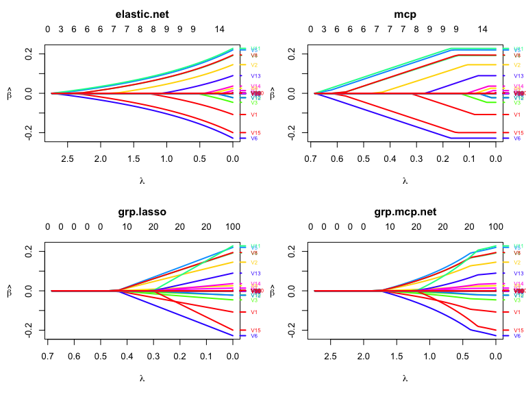
These binaries (installable software) and packages are in development.
They may not be fully stable and should be used with caution. We make no claims about them.
Health stats visible at Monitor.