The hardware and bandwidth for this mirror is donated by dogado GmbH, the Webhosting and Full Service-Cloud Provider. Check out our Wordpress Tutorial.
If you wish to report a bug, or if you are interested in having us mirror your free-software or open-source project, please feel free to contact us at mirror[@]dogado.de.
The goal of nlmixr2plot is to provide the nlmixr2 core estimation routines.
You can install the development version of nlmixr2plot from GitHub with:
# install.packages("remotes")
remotes::install_github("nlmixr2/nlmixr2data")
remotes::install_github("nlmixr2/lotri")
remotes::install_github("nlmixr2/rxode2")
remotes::install_github("nlmixr2/nlmixr2est")
remotes::install_github("nlmixr2/nlmixr2extra")
remotes::install_github("nlmixr2/nlmixr2plot")
For most people, using nlmixr2 directly would be likely easier.
library(nlmixr2est)
#> Loading required package: nlmixr2data
library(nlmixr2plot)

## The basic model consists of an ini block that has initial estimates
one.compartment <- function() {
  ini({
    tka <- 0.45 ; label("Log Ka")
    tcl <- 1 ; label("Log Cl")
    tv <- 3.45 ; label("Log V")
    eta.ka ~ 0.6
    eta.cl ~ 0.3
    eta.v ~ 0.1
    add.sd <- 0.7
  })
  # and a model block with the error specification and model specification
  model({
    ka <- exp(tka + eta.ka)
    cl <- exp(tcl + eta.cl)
    v <- exp(tv + eta.v)
    d/dt(depot) = -ka * depot
    d/dt(center) = ka * depot - cl / v * center
    cp = center / v
    cp ~ add(add.sd)
  })
}

## The fit is performed by the function nlmixr/nlmix2 specifying the model, data and estimate
fit <- nlmixr2(one.compartment, theo_sd,  est="saem", saemControl(print=0))
#> → loading into symengine environment...
#> → pruning branches (`if`/`else`) of saem model...
#> ✔ done
#> → finding duplicate expressions in saem model...
#> [====|====|====|====|====|====|====|====|====|====] 0:00:00
#> → optimizing duplicate expressions in saem model...
#> [====|====|====|====|====|====|====|====|====|====] 0:00:00
#> ✔ done
#> rxode2 2.0.11.9000 using 8 threads (see ?getRxThreads)
#>   no cache: create with `rxCreateCache()`
#> Calculating covariance matrix
#> → loading into symengine environment...
#> → pruning branches (`if`/`else`) of saem model...
#> ✔ done
#> → finding duplicate expressions in saem predOnly model 0...
#> → finding duplicate expressions in saem predOnly model 1...
#> → optimizing duplicate expressions in saem predOnly model 1...
#> → finding duplicate expressions in saem predOnly model 2...
#> ✔ done
#> → Calculating residuals/tables
#> ✔ done
#> → compress origData in nlmixr2 object, save 5952
#> → compress phiM in nlmixr2 object, save 62360
#> → compress parHist in nlmixr2 object, save 9592
#> → compress saem0 in nlmixr2 object, save 28760

print(fit)
#> ── nlmixr² SAEM OBJF by FOCEi approximation ──
#>
#>  Gaussian/Laplacian Likelihoods: AIC() or $objf etc.
#>  FOCEi CWRES & Likelihoods: addCwres()
#>
#> ── Time (sec $time): ──
#>
#>         setup covariance saem table compress other
#> elapsed 0.002       0.01 5.24   0.1     0.09 2.498
#>
#> ── Population Parameters ($parFixed or $parFixedDf): ──
#>
#>        Parameter  Est.     SE %RSE Back-transformed(95%CI) BSV(CV%) Shrink(SD)%
#> tka       Log Ka 0.454  0.196 43.1       1.57 (1.07, 2.31)     71.5   -0.0203%
#> tcl       Log Cl  1.02 0.0853  8.4       2.76 (2.34, 3.26)     27.6      3.46%
#> tv         Log V  3.45 0.0454 1.32       31.5 (28.8, 34.4)     13.4      9.89%
#> add.sd           0.693                               0.693
#>
#>   Covariance Type ($covMethod): linFim
#>   No correlations in between subject variability (BSV) matrix
#>   Full BSV covariance ($omega) or correlation ($omegaR; diagonals=SDs)
#>   Distribution stats (mean/skewness/kurtosis/p-value) available in $shrink
#>   Censoring ($censInformation): No censoring
#>
#> ── Fit Data (object is a modified tibble): ──
#> # A tibble: 132 × 19
#>   ID     TIME    DV  PRED    RES IPRED   IRES  IWRES eta.ka eta.cl   eta.v    cp
#>   <fct> <dbl> <dbl> <dbl>  <dbl> <dbl>  <dbl>  <dbl>  <dbl>  <dbl>   <dbl> <dbl>
#> 1 1      0     0.74  0     0.74   0     0.74   1.07   0.103 -0.491 -0.0820  0
#> 2 1      0.25  2.84  3.27 -0.426  3.87 -1.03  -1.48   0.103 -0.491 -0.0820  3.87
#> 3 1      0.57  6.57  5.85  0.723  6.82 -0.246 -0.356  0.103 -0.491 -0.0820  6.82
#> # … with 129 more rows, and 7 more variables: depot <dbl>, center <dbl>,
#> #   ka <dbl>, cl <dbl>, v <dbl>, tad <dbl>, dosenum <dbl>

# this now gives the goodness of fit plots
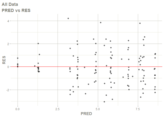
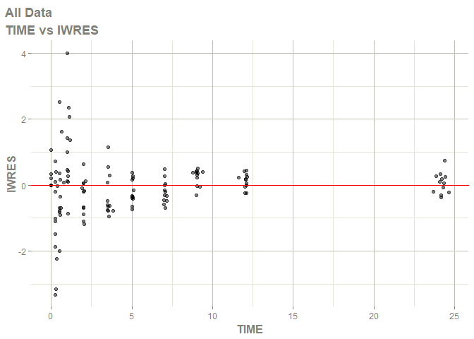
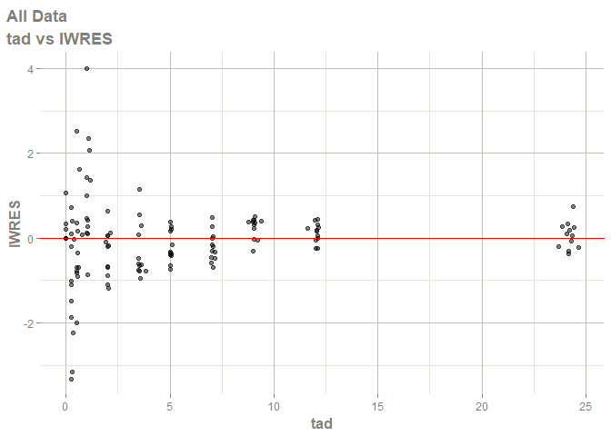
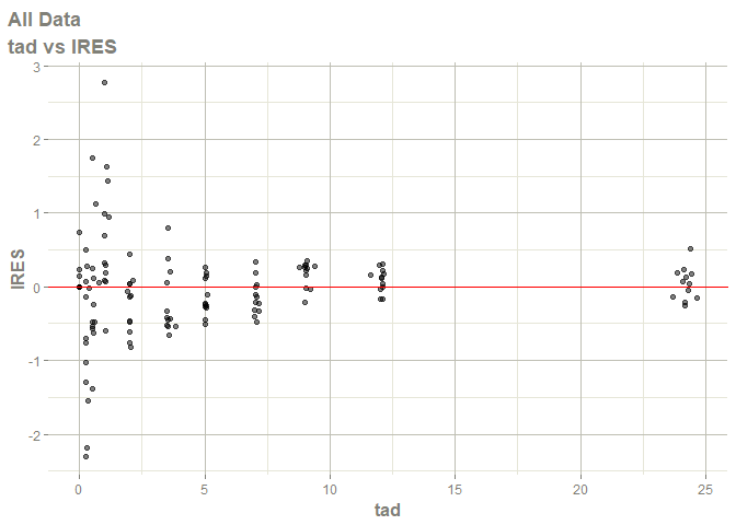
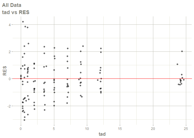
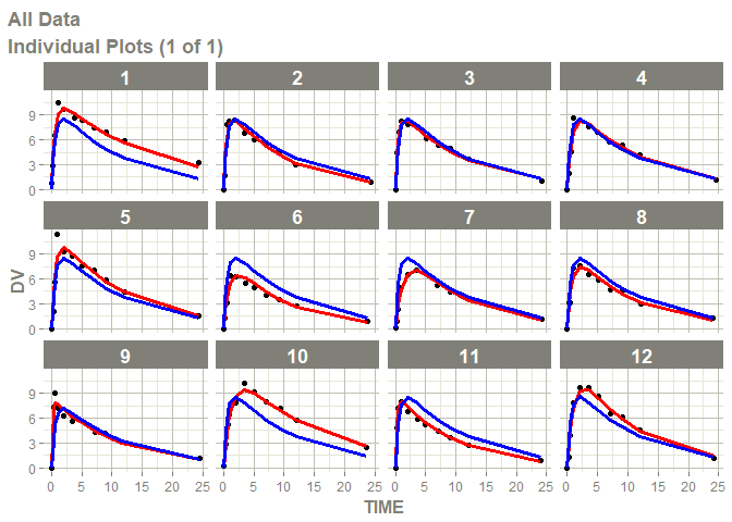
plot(fit)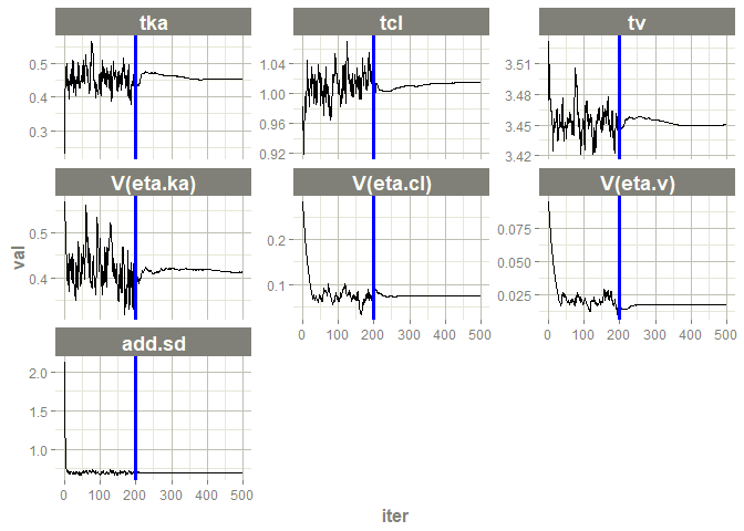
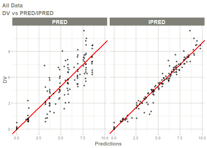
#> Warning: Transformation introduced infinite values in continuous x-axis
#> Warning: Transformation introduced infinite values in continuous y-axis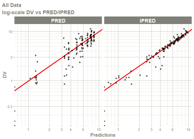
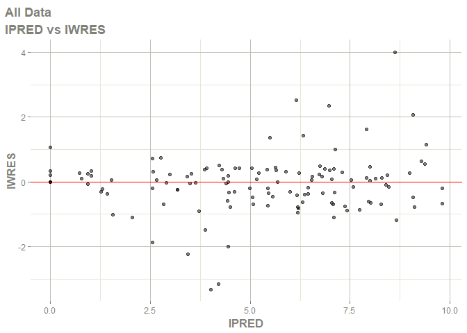
#> Warning: Transformation introduced infinite values in continuous x-axis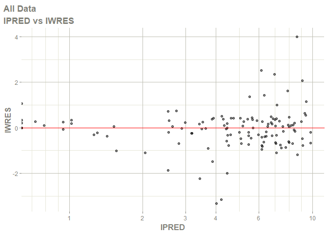
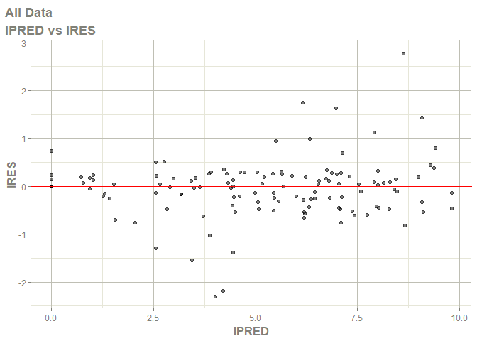
#> Warning: Transformation introduced infinite values in continuous x-axis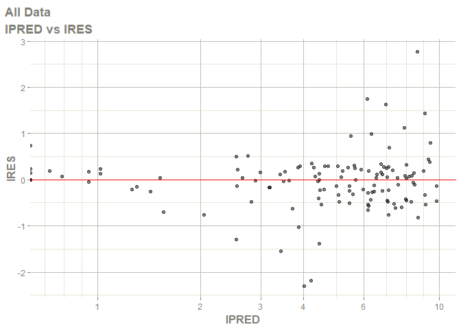
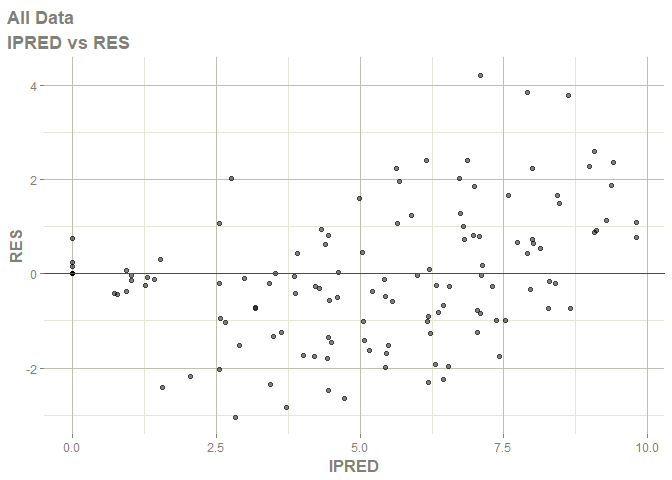
#> Warning: Transformation introduced infinite values in continuous x-axis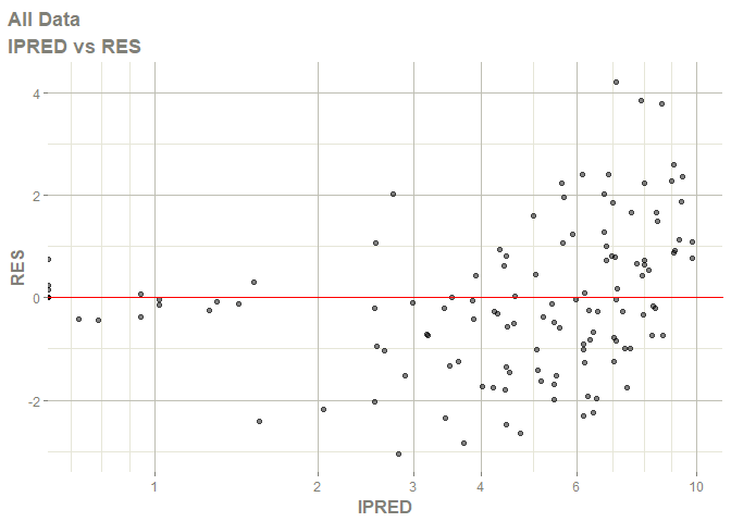
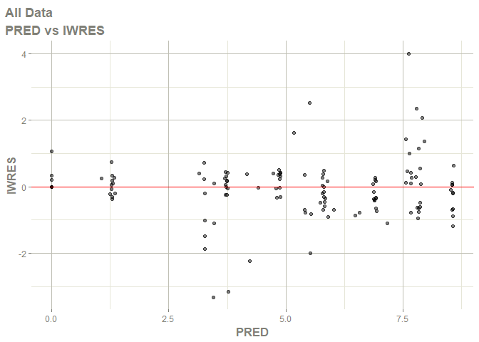
#> Warning: Transformation introduced infinite values in continuous x-axis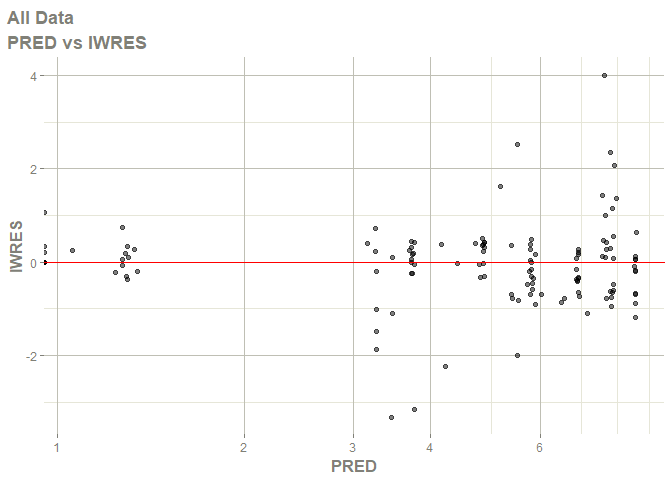
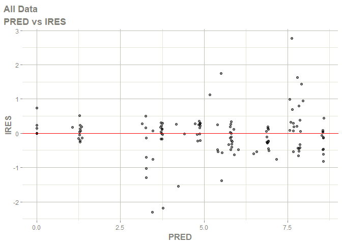
#> Warning: Transformation introduced infinite values in continuous x-axis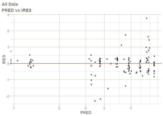
#> Warning: Transformation introduced infinite values in continuous x-axis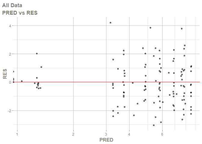
#> Warning: Transformation introduced infinite values in continuous x-axis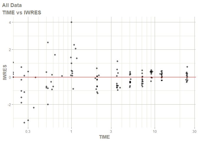
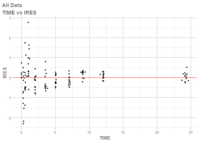
#> Warning: Transformation introduced infinite values in continuous x-axis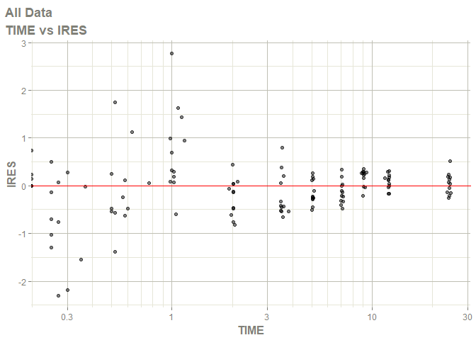
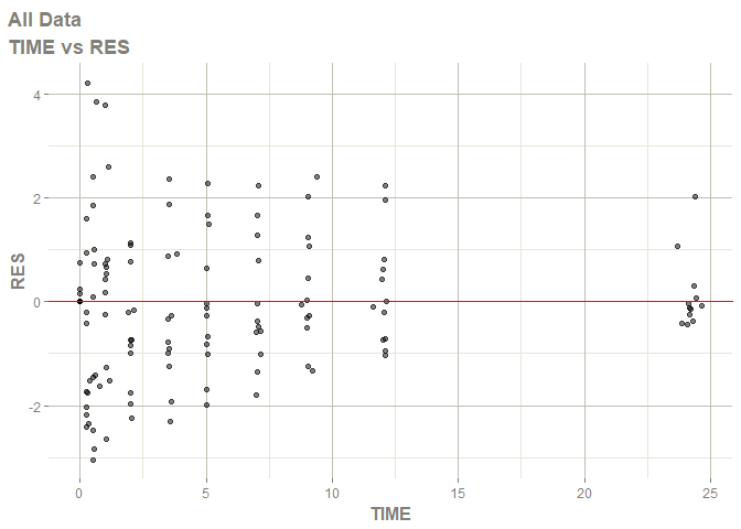
#> Warning: Transformation introduced infinite values in continuous x-axis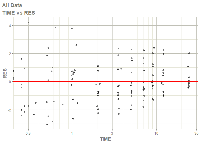
#> Warning: Transformation introduced infinite values in continuous x-axis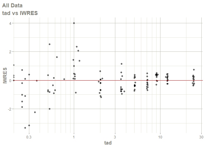
#> Warning: Transformation introduced infinite values in continuous x-axis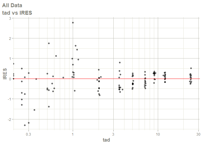
#> Warning: Transformation introduced infinite values in continuous x-axis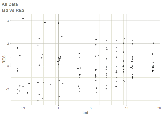
These binaries (installable software) and packages are in development.
They may not be fully stable and should be used with caution. We make no claims about them.
Health stats visible at Monitor.