The hardware and bandwidth for this mirror is donated by dogado GmbH, the Webhosting and Full Service-Cloud Provider. Check out our Wordpress Tutorial.
If you wish to report a bug, or if you are interested in having us mirror your free-software or open-source project, please feel free to contact us at mirror[@]dogado.de.

netplot

netplot is a graph visualization engine for R that emphasizes aesthetics. Its defaults are chosen so that a single call to nplot() produces a publication-quality figure out of the box, while still giving you fine-grained control when you need it. It works directly with igraph, network, and adjacency-matrix objects.

Why netplot?

Compared with the base plot() methods in igraph and sna/network, netplot aims to make the common case beautiful and the hard case possible:

• Beautiful defaults. Vertices, edges, arrows, and labels are auto-scaled relative to the plotting device, so figures look right regardless of size or aspect ratio and fill the plotting area instead of floating in whitespace.
• Map data to aesthetics with formulas. Color, shape, and size vertices (and scale edge widths) straight from graph attributes: nplot(g, vertex.color = ~ group, vertex.nsides = ~ group, vertex.size = ~ degree). Categorical, numeric, and logical attributes are each handled sensibly, and a legend is added automatically. See vignette("formulas").
• Smart edges. True curved edges with user-defined curvature, an embedded edge-color mixer that blends each edge between its endpoints’ colors, and edge-width/arrow scaling that respects the layout.
• Built on grid. Because netplot draws with the grid system (the same engine as ggplot2), plots are first-class grid objects: you can post-edit them with set_vertex_gpar() / set_edge_gpar(), arrange several with gridExtra::grid.arrange(), add gradients, and export cleanly.
• Lightweight. Following the “tinyverse” philosophy, netplot leans on base R graphics facilities and keeps its dependency footprint small.

A quick feature checklist:

1. Auto-scaling of vertices, edges, and labels relative to the plotting device.
2. Formula interface to map colors, shapes, and sizes from graph attributes.
3. Embedded edge color mixer (blends edges between endpoint colors).
4. True curved edges with user-defined curvature.
5. Nicer vertex frame colors and vertex shapes.
6. Automatic legends and color keys.
7. Gradient fills for vertices and edges.
8. Better use of space, filling the plotting device.

The package uses the grid plotting system (just like ggplot2).

Installation

You can install the released version of netplot from CRAN with:

install.packages("netplot")

And the development version from GitHub with:

# install.packages("devtools")
devtools::install_github("USCCANA/netplot")

Example

This is a basic example which shows you how to solve a common problem:

library(igraph)
#> 
#> Attaching package: 'igraph'
#> The following objects are masked from 'package:stats':
#> 
#>     decompose, spectrum
#> The following object is masked from 'package:base':
#> 
#>     union
library(netplot)
#> Loading required package: grid
#> 
#> Attaching package: 'netplot'
#> The following object is masked from 'package:igraph':
#> 
#>     ego
set.seed(1)
data("UKfaculty", package = "igraphdata")
l <- layout_with_fr(UKfaculty)
#> This graph was created by an old(er) igraph version.
#> ℹ Call `igraph::upgrade_graph()` on it to use with the current igraph version.
#> For now we convert it on the fly...

plot(UKfaculty, layout = l) # ala igraph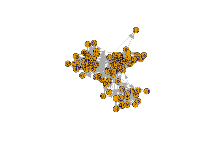

V(UKfaculty)$ss <- runif(vcount(UKfaculty))
nplot(UKfaculty, layout = l) # ala netplot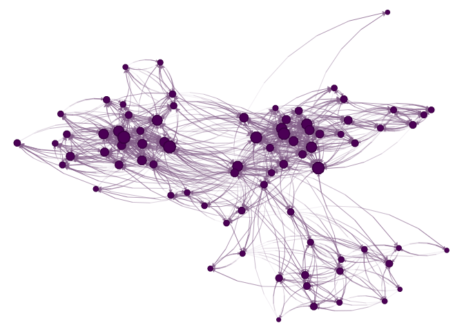

sna::gplot(intergraph::asNetwork(UKfaculty), coord=l)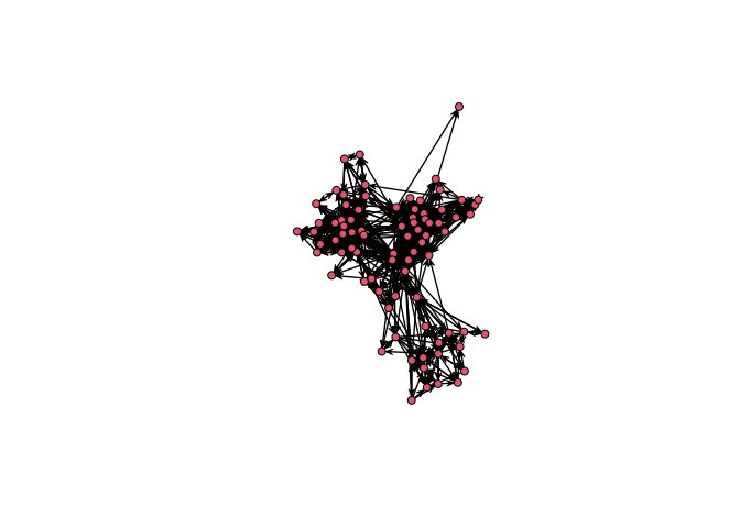

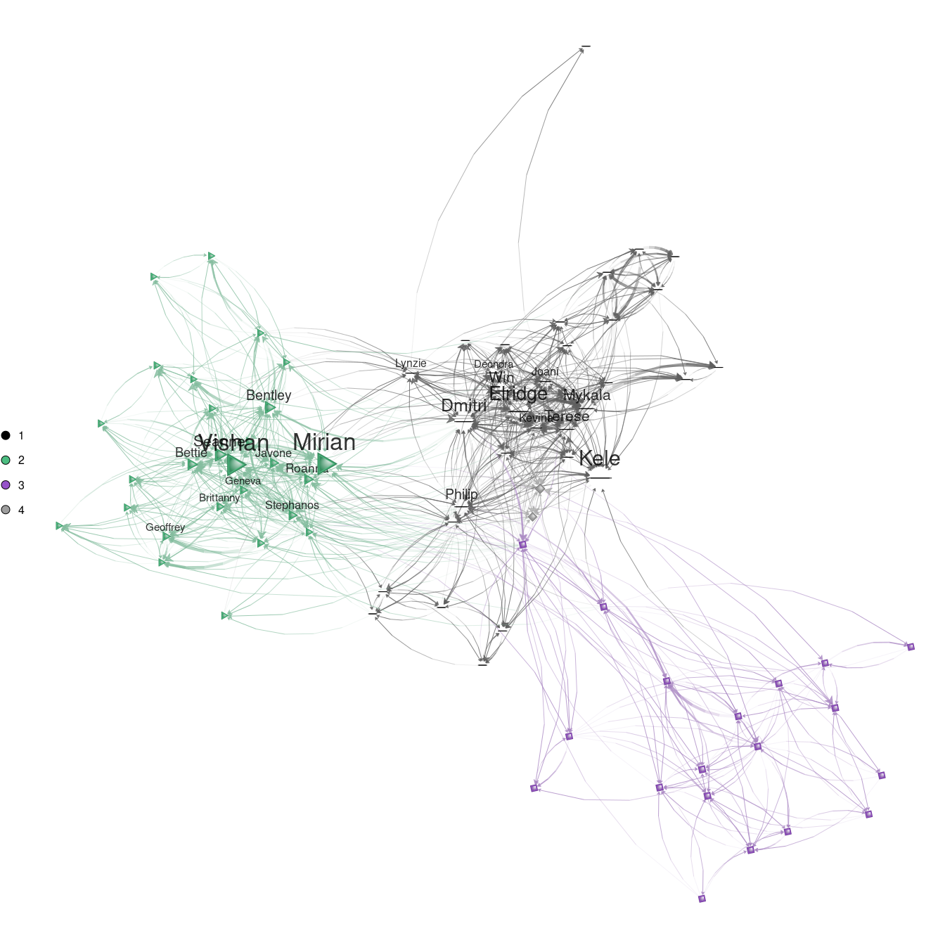
UKfaculty

# Random names
set.seed(1)
nam <- sample(babynames::babynames$name, vcount(UKfaculty))

ans <- nplot(
  UKfaculty,
  layout                = l,
  vertex.color          = ~ Group,
  vertex.nsides         = ~ Group,
  vertex.label          = nam,
  vertex.size.range     = c(.01, .03, 4),
  bg.col                = "transparent",
  vertex.label.show     = .25,
  vertex.label.range    = c(10, 25),
  edge.width.range      = c(1, 4, 5),
  vertex.label.fontfamily = "sans"
  )

# Plot it!
ans

Starting version 0.2-0, we can use gradients!

ans |>
  set_vertex_gpar(
    element = "core",
    fill = lapply(get_vertex_gpar(ans, "frame", "col")$col, \(i) {
      radialGradient(c("white", i), cx1=.8, cy1=.8, r1=0)
      }))

USairports

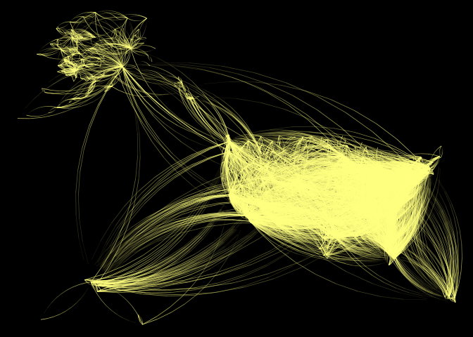
# Loading the data
data(USairports, package="igraphdata")

# Generating a layout naively
layout   <- V(USairports)$Position
#> This graph was created by an old(er) igraph version.
#> ℹ Call `igraph::upgrade_graph()` on it to use with the current igraph version.
#> For now we convert it on the fly...
layout   <- do.call(rbind, lapply(layout, function(x) strsplit(x, " ")[[1]]))
layout[] <- stringr::str_remove(layout, "^[a-zA-Z]+")
layout   <- matrix(as.numeric(layout[]), ncol=2)

# Some missingness
layout[which(!complete.cases(layout)), ] <- apply(layout, 2, mean, na.rm=TRUE)

# Have to rotate it (it doesn't matter the origin)
layout <- netplot:::rotate(layout, c(0,0), pi/2)

# Simplifying the network
net <- simplify(USairports, edge.attr.comb = list(
  weight = "sum",
  name   = "concat",
  Passengers = "sum",
  "ignore"
))

# Pretty graph
nplot(
  net,
  layout            = layout,
  edge.width        = ~ Passengers,
  edge.color        = ~
    ego(col = "white", alpha = 0) +
    alter(col = "yellow", alpha = .75),
  skip.vertex       = TRUE,
  skip.arrows       = TRUE,
  edge.width.range  = c(.75, 4, 4), 
  bg.col            = "black",
  edge.line.breaks  = 10
  )

These binaries (installable software) and packages are in development.
They may not be fully stable and should be used with caution. We make no claims about them.
Health stats visible at Monitor.