The hardware and bandwidth for this mirror is donated by dogado GmbH, the Webhosting and Full Service-Cloud Provider. Check out our Wordpress Tutorial.
If you wish to report a bug, or if you are interested in having us mirror your free-software or open-source project, please feel free to contact us at mirror[@]dogado.de.

msPCA

Sparse PCA with multiple principal components in R.

The msPCA package computes sparse loading vectors that explain a high fraction of variance while controlling non-redundancy across components. It supports two non-redundancy definitions:

• orthogonality of loading vectors,
• zero pairwise correlation of components.

Installation

Install from CRAN:

install.packages("msPCA")
library(msPCA)

Install development version from GitHub:

install.packages("devtools")
devtools::install_github("jeanpauphilet/msPCA")
library(msPCA)

Quick start

The main function is mspca().

Inputs (following the elasticnet convention, the data is a single argument M plus a type selector):

• M: the data matrix,
• type: "Sigma" (default) treats M as a covariance/correlation matrix (p x p); "X" treats M as a raw data matrix (n observations x p variables),
• r: number of sparse principal components,
• ks: integer vector of length r with sparsity budgets.

With type = "X", mspca() applies the algorithm to the data directly via the products t(X) %*% (X %*% beta) and never forms the p x p matrix. This is substantially faster and more memory-efficient when n << p. Pass type = "X" whenever the number of variables greatly exceeds the number of observations.

Output fields:

• x_best: sparse loading matrix (p x r),
• objective_value,
• feasibility_violation,
• runtime.

Example on mtcars:

library(msPCA)

Sigma <- cor(datasets::mtcars)
set.seed(42)

res <- mspca(Sigma, r = 2, ks = c(4, 4), verbose = FALSE)   # type = "Sigma" is the default
print_mspca(res, Sigma)

feasibility_violation_off(Sigma, res$x_best, feasibilityConstraintType = 0)
fraction_variance_explained(Sigma, res$x_best)

Equivalent workflow from the raw data matrix (no covariance matrix needed):

library(msPCA)

X <- as.matrix(datasets::mtcars)
set.seed(42)

# type = "X" treats the first argument as raw data; scale = TRUE operates on the
# correlation matrix, matching cor(mtcars) above.
res <- mspca(X, r = 2, ks = c(4, 4), type = "X", scale = TRUE, verbose = FALSE)
print_mspca(res)                      # type = "X" results carry their own variance summary

fraction_variance_explained(cor(X), res$x_best)

For datasets with n << p, this raw-data path avoids the O(np^2) cost of forming Sigma and reduces each iteration’s matrix–vector product from O(p^2) to O(np).

Optional dense PCA comparison:

pca_res <- prcomp(datasets::mtcars, scale. = TRUE)
fraction_variance_explained(Sigma, pca_res$rotation[, 1:2])

Interpretation:

• Dense PCA usually explains more variance.
• Sparse PCA improves interpretability by restricting each component to a small set of features.

See vignette("msPCA") for a worked example built from the same mtcars workflow.

Synthetic benchmark

The script test/notebook_synthetic.R compares msPCA with elasticnet::spca() on synthetic data across sample sizes and exports the figures below.

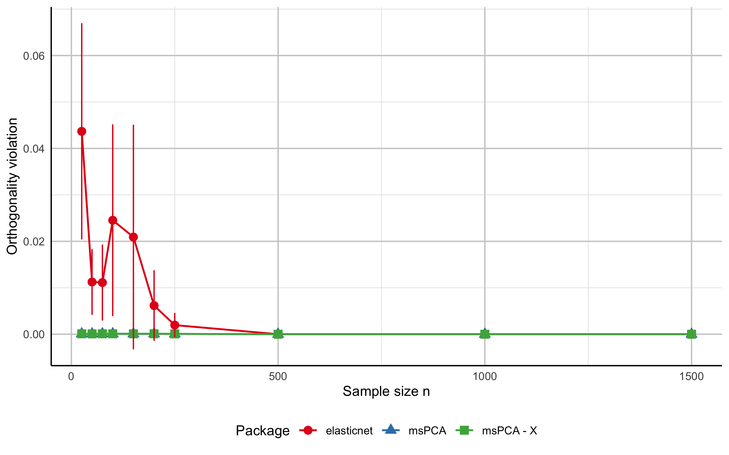
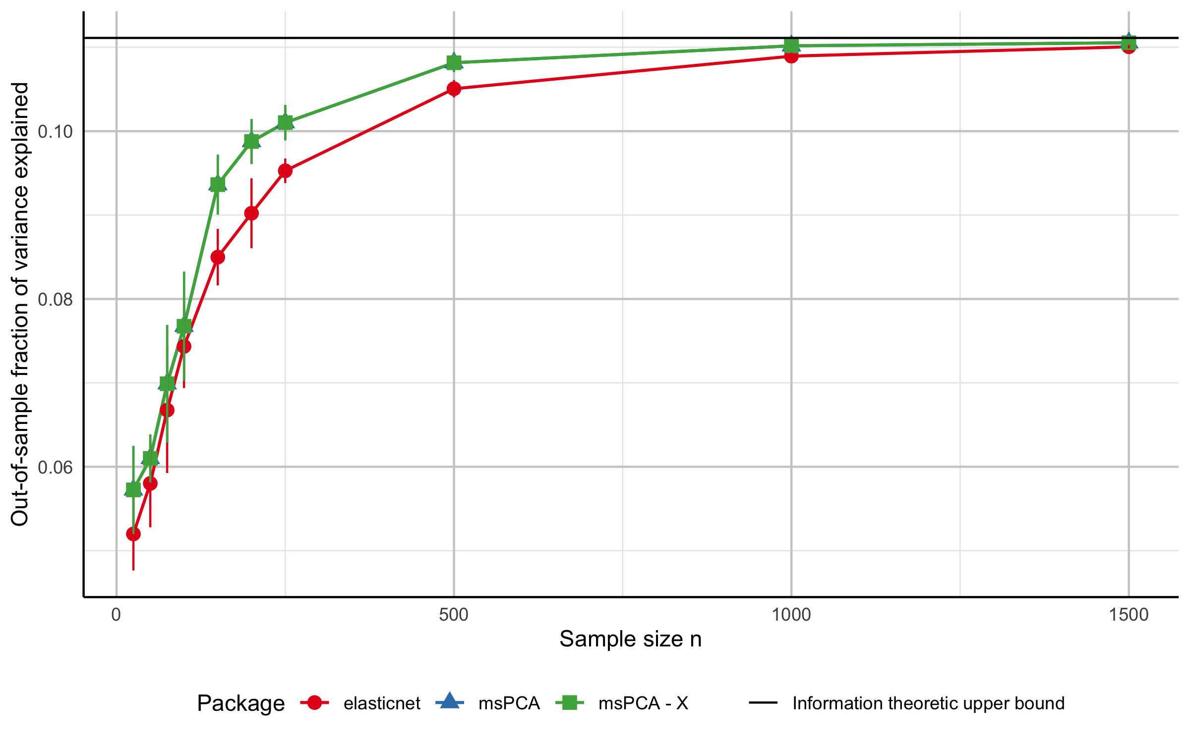
To regenerate these files, run test/notebook_synthetic.R from the repository root.

Choosing parameters

Sparsity budgets (ks)

ks is the main tuning input. A practical workflow is to run mspca() for multiple sparsity budgets and evaluate:

• fraction of variance explained (fraction_variance_explained()),
• feasibility violation (feasibility_violation_off()),
• interpretability of nonzero loadings.

Constraint type (feasibilityConstraintType)

• 0 (default): orthogonality constraints on loading vectors.
• 1: zero pairwise correlation constraints on components.

Use 0 when loadings are used as a geometric projection basis. Use 1 when statistical decorrelation of component scores is the priority.

Main functions

• mspca(M, r, ks, type = c("Sigma", "X"), ...): multiple sparse PCs.
• tpm(M, k, type = c("Sigma", "X"), ...): single sparse PC via truncated power method.

Useful optional arguments in mspca():

• feasibilityConstraintType
• feasibilityTolerance
• maxIter
• stallingTolerance
• timeLimitTPM
• maxRestartTPM
• minRestartTPM

Raw-data arguments (type = "X"):

• center (default TRUE), scale (default TRUE, set FALSE for covariance),
• divisor ("n-1" for the sample covariance, the default, or "n").

Covariance-matrix validation arguments (type = "Sigma"):

• checkPSD (default TRUE), symTolerance, psdTolerance.

Diagnostic functions

• fraction_variance_explained(Sigma, U)
• fraction_variance_explained_perPC(Sigma, U)
• variance_explained_perPC(Sigma, U)
• feasibility_violation_off(Sigma, U, feasibilityConstraintType)
• print_mspca(sol_object, Sigma, digits = 3)

Citation

If you use msPCA in academic work, please cite the package and the underlying paper.

You can retrieve the package citation in R with:

citation("msPCA")

Reference paper:

@article{cory2026sparse,
  title   = {Sparse PCA with Multiple Principal Components},
  author  = {Cory-Wright, Ryan and Pauphilet, Jean},
  year    = {2026},
  journal = {Operations Research},
  doi     = {10.1287/opre.2023.0598}
}

Development

Package structure overview:

• R/
  • main.R: user-facing functions and helper diagnostics.
  • RcppExports.R: R interface for compiled code (typically generated with Rcpp::compileAttributes()).
• src/
  • msPCA_R_CPP.cpp: C++ implementation of the core algorithm and the dense/raw-data entry points.
  • CovOperator.h: covariance-operator abstraction (DenseOp for Sigma, GramOp for X).
  • ConstantArguments.h: internal algorithm constants.
  • RcppExports.cpp: generated C++ interface.
  • Makevars, Makevars.win: compilation settings.
• man/: function documentation generated from roxygen comments.
• test/
  • notebook_mtcars.R
  • notebook_plot.R
  • notebook_synthetic.R
  • msPCA_synthetic_results.csv

For interface changes, regenerate exports and documentation with Rcpp::compileAttributes() and devtools::document().

License

See LICENSE.

These binaries (installable software) and packages are in development.
They may not be fully stable and should be used with caution. We make no claims about them.
Health stats visible at Monitor.