
The hardware and bandwidth for this mirror is donated by dogado GmbH, the Webhosting and Full Service-Cloud Provider. Check out our Wordpress Tutorial.
If you wish to report a bug, or if you are interested in having us mirror your free-software or open-source project, please feel free to contact us at mirror[@]dogado.de.
The mrangr package is designed to simulate
metacommunities within a spatially explicit, mechanistic
framework. It extends the functionality of the rangr package
by allowing for the simulation of multiple interacting
species via an asymmetric interaction matrix.
This tool mimics the essential processes shaping metacommunity dynamics: local population growth, dispersal, and interspecific interactions. Simulations take place in dynamic environments, facilitating projections of community shifts in response to environmental changes.
You can install mrangr with:
install.packages("mrangr")The mrangr workflow involves initialising a community
with spatial data and interaction parameters, running the simulation,
and analysing the results.
You must provide carrying capacity maps (K_map) and
initial abundance maps (n1_map) as SpatRaster
objects. For a community of \(N\)
species, the rasters must contain \(N\)
layers.
# Load example maps
K_map <- rast(system.file("input_maps/K_map_eg.tif", package = "mrangr"))
K_map <- subset(K_map, 1:2)
Interspecific interactions are defined using an interaction matrix (\(a\)), where values represent the per-capita interaction strength of the species in the column on the species in the row.
# Example for 2 species with symmetric competition
nspec <- 2
a <- matrix(c(NA, -0.8, -0.8, NA), nrow = nspec, ncol = nspec)Use initialise_com() to create a
sim_com_data object. This stores all parameters, including
the intrinsic growth rate (\(r\)) and
the dispersal rate.
first_com <- initialise_com(
  n1_map = round(K_map / 2),
  K_map = K_map,
  r = 1.1,
  a = a,
  rate = 1 / 500
)The sim_com() function executes the simulation over a
specified number of time steps.
first_sim <- sim_com(first_com, time = 100)You can visualise the final spatial distributions or the change in mean abundance over time.
# Visualise spatial niches at specific time steps
plot(first_sim, time = c(1, 10, 100))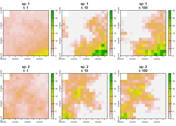
# Plot abundance time series for all species
plot_series(first_sim)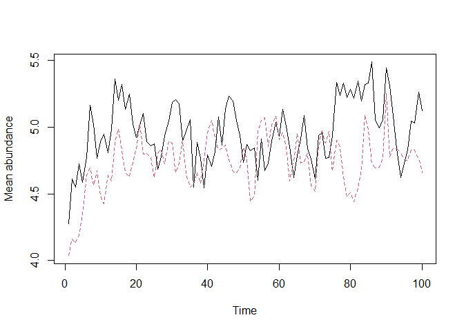
The package includes a virtual_ecologist() function to
simulate real-world observation processes. This allows users to sample
the simulated community at defined points in space and time,
incorporating sampling effort and detection probability into the
simulation.
To cite mrangr, please use the
citation() function:
library(mrangr)
citation("mrangr")
These binaries (installable software) and packages are in development.
They may not be fully stable and should be used with caution. We make no claims about them.
Health stats visible at Monitor.