The hardware and bandwidth for this mirror is donated by dogado GmbH, the Webhosting and Full Service-Cloud Provider. Check out our Wordpress Tutorial.
If you wish to report a bug, or if you are interested in having us mirror your free-software or open-source project, please feel free to contact us at mirror[@]dogado.de.
The goal of mlspatial is to …
You can install the development version of mlspatial from GitHub with:
# install.packages("mlspatial")
mlspatial::mlspatial("azizadeboye/mlspatial")This is a basic example which shows you how to solve a common problem:
library(mlspatial)
#> Loading required package: tidyverse
#> ── Attaching core tidyverse packages ──────────────────────── tidyverse 2.0.0 ──
#> ✔ dplyr     1.1.4     ✔ readr     2.1.5
#> ✔ forcats   1.0.0     ✔ stringr   1.5.1
#> ✔ ggplot2   3.5.2     ✔ tibble    3.3.0
#> ✔ lubridate 1.9.4     ✔ tidyr     1.3.1
#> ✔ purrr     1.0.4
#> ── Conflicts ────────────────────────────────────────── tidyverse_conflicts() ──
#> ✖ dplyr::filter() masks stats::filter()
#> ✖ dplyr::lag()    masks stats::lag()
#> ℹ Use the conflicted package (<http://conflicted.r-lib.org/>) to force all conflicts to become errors
## basic example code
What is special about using README.Rmd instead of just
README.md? You can include R chunks like so:
knitr::opts_chunk$set(echo = TRUE, message = FALSE, warning = FALSE)
library(mlspatial)
library(dplyr)
library(ggplot2)
library(tmap)
library(sf)
#> Linking to GEOS 3.13.0, GDAL 3.8.5, PROJ 9.5.1; sf_use_s2() is TRUE
library(spdep)
#> Loading required package: spData
#> To access larger datasets in this package, install the spDataLarge
#> package with: `install.packages('spDataLarge',
#> repos='https://nowosad.github.io/drat/', type='source')`
library(rgeoda)
#> Loading required package: digest
#>
#> Attaching package: 'rgeoda'
#> The following object is masked from 'package:spdep':
#>
#>     skater
library(gstat)
library(randomForest)
#> randomForest 4.7-1.2
#> Type rfNews() to see new features/changes/bug fixes.
#>
#> Attaching package: 'randomForest'
#> The following object is masked from 'package:dplyr':
#>
#>     combine
#> The following object is masked from 'package:ggplot2':
#>
#>     margin
library(xgboost)
#>
#> Attaching package: 'xgboost'
#> The following object is masked from 'package:dplyr':
#>
#>     slice
library(e1071)
library(caret)
#> Loading required package: lattice
#>
#> Attaching package: 'caret'
#> The following object is masked from 'package:purrr':
#>
#>     lift
# Join data
mapdata <- join_data(africa_shp, panc_incidence, by = "NAME")
## OR Joining/ merging my data and shapefiles
mapdata <- inner_join(africa_shp, panc_incidence, by = "NAME")
## OR mapdata <- left_join(nat, codata, by = "DISTRICT_N")
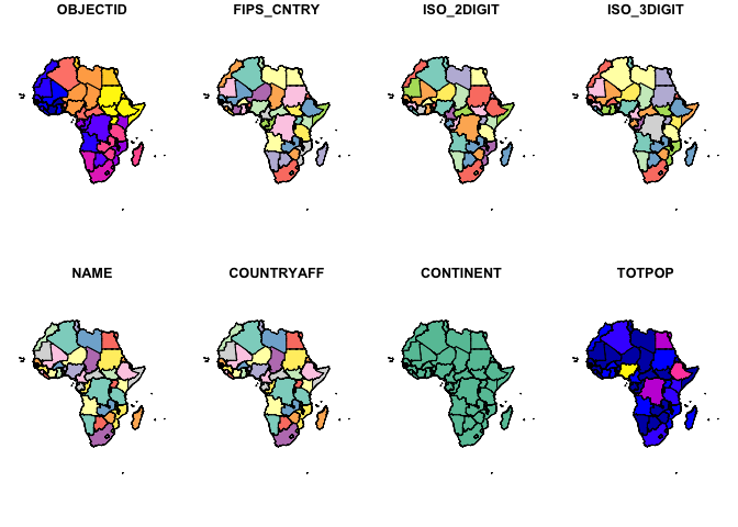
str(mapdata)
#> Classes 'sf' and 'data.frame': 53 obs. of 26 variables:
#> $ OBJECTID : int 2 3 5 6 7 8 9 10 11 12 ...
#> $ FIPS_CNTRY: chr "UV" "CV" "GA" "GH" ...
#> $ ISO_2DIGIT: chr "BF" "CV" "GM" "GH" ...
#> $ ISO_3DIGIT: chr "BFA" "CPV" "GMB" "GHA" ...
#> $ NAME : chr "Burkina Faso" "Cabo Verde" "Gambia" "Ghana" ...
#> $ COUNTRYAFF: chr "Burkina Faso" "Cabo Verde" "Gambia" "Ghana" ...
#> $ CONTINENT : chr "Africa" "Africa" "Africa" "Africa" ...
#> $ TOTPOP : int 20107509 560899 2051363 27499924 12413867 1792338 4689021 17885245 3758571 33986655 ...
#> $ incidence : num 330.4 53.4 31.4 856.3 163.1 ...
#> $ female : num 1683 362 140 4566 375 ...
#> $ male : num 1869 211 197 4640 1378 ...
#> $ ageb : num 669.7 93.7 68.7 2047 336.7 ...
#> $ agec : num 2878 480 268 7147 1414 ...
#> $ agea : num 4.597 0.265 0.718 11.888 2.13 ...
#> $ fageb : num 250.3 40.2 23.1 782 59.1 ...
#> $ fagec : num 1429 322 116 3775 315 ...
#> $ fagea : num 3.413 0.146 0.548 8.816 1.228 ...
#> $ mageb : num 419.5 53.5 45.6 1265 277.6 ...
#> $ magec : num 1448 158 152 3372 1100 ...
#> $ magea : num 1.184 0.12 0.17 3.073 0.902 ...
#> $ yra : num 182.4 30.2 16.6 524.7 73.1 ...
#> $ yrb : num 187.2 34.1 17.1 552.6 74.9 ...
#> $ yrc : num 193.1 35 18 578.5 76.9 ...
#> $ yrd : num 198.5 35.9 18.3 602.7 78.6 ...
#> $ yre : num 204.3 36.5 18.7 621.5 79.4 ...
#> $ geometry :sfc_MULTIPOLYGON of length 53; first list element: List of 1
#> ..$ :List of 1
#> .. ..$ : num [1:317, 1:2] 102188 90385 80645 74151 70224 ...
#> ..- attr(*, "class")= chr [1:3] "XY" "MULTIPOLYGON" "sfg"
#> - attr(*, "sf_column")= chr "geometry"
#> - attr(*, "agr")= Factor w/ 3 levels "constant","aggregate",..: NA NA NA NA NA NA NA NA NA NA ...
#> ..- attr(*, "names")= chr [1:25] "OBJECTID" "FIPS_CNTRY" "ISO_2DIGIT" "ISO_3DIGIT" ...#Visualize Pancreatic cancer Incidence by countries
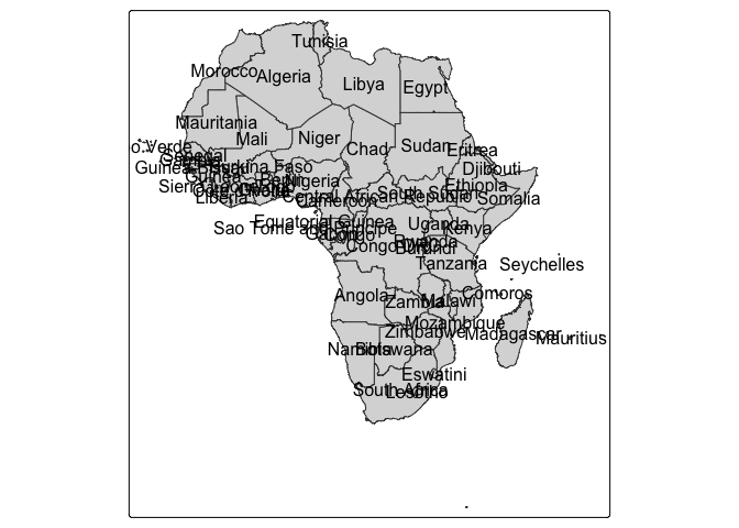
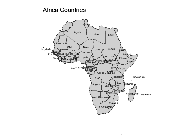
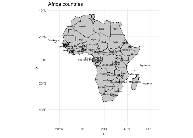
#Basic map with labels
# quantile map
p1 <- tm_shape(mapdata) +
tm_fill("incidence", fill.scale =tm_scale_intervals(values = "brewer.reds", style = "quantile"),
fill.legend = tm_legend(title = "Incidence")) + tm_borders(fill_alpha = .3) + tm_compass() +
tm_layout(legend.text.size = 0.5, legend.position = c("left", "bottom"), frame = TRUE, component.autoscale = FALSE)
p2 <- tm_shape(mapdata) +
tm_fill("female", fill.scale =tm_scale_intervals(values = "brewer.reds", style = "quantile"),
fill.legend = tm_legend(title = "Female")) + tm_borders(fill_alpha = .3) + tm_compass() +
tm_layout(legend.text.size = 0.5, legend.position = c("left", "bottom"), frame = TRUE, component.autoscale = FALSE)
current.mode <- tmap_mode("plot")
tmap_arrange(p1, p2, widths = c(.75, .75))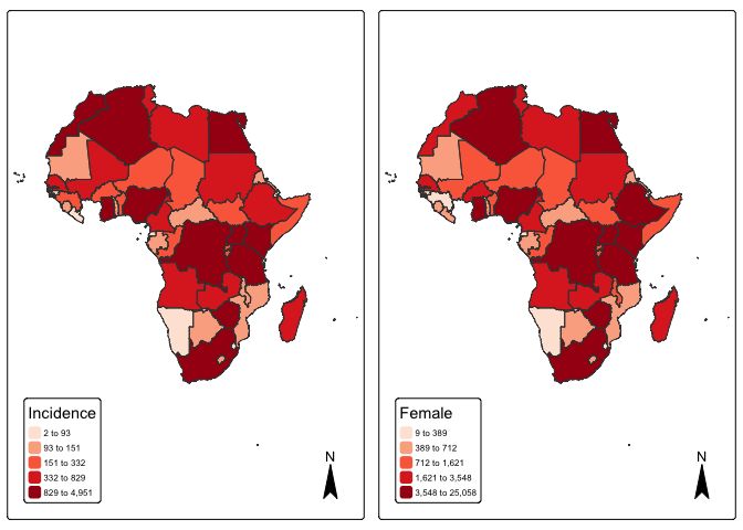
tmap_mode(current.mode)These binaries (installable software) and packages are in development.
They may not be fully stable and should be used with caution. We make no claims about them.
Health stats visible at Monitor.