The hardware and bandwidth for this mirror is donated by dogado GmbH, the Webhosting and Full Service-Cloud Provider. Check out our Wordpress Tutorial.
If you wish to report a bug, or if you are interested in having us mirror your free-software or open-source project, please feel free to contact us at mirror[@]dogado.de.

![]()
![]()
![]()

melt provides a unified framework for data analysis with empirical likelihood methods. A collection of functions is available to perform multiple empirical likelihood tests and construct confidence intervals for various models in ‘R’. melt offers an easy-to-use interface and flexibility in specifying hypotheses and calibration methods, extending the framework to simultaneous inferences. The core computational routines are implemented with the ‘Eigen’ ‘C++’ library and ‘RcppEigen’ interface, with ‘OpenMP’ for parallel computation. Details of the testing procedures are provided in Kim, MacEachern, and Peruggia (2023). The package has a companion paper by Kim, MacEachern, and Peruggia (2024). This work was supported by the U.S. National Science Foundation under Grants No. SES-1921523 and DMS-2015552.
You can install the latest stable release of melt from CRAN.
install.packages("melt")You can install the development version of melt from GitHub or R-universe.
# install.packages("pak")
pak::pak("ropensci/melt")install.packages("melt", repos = "https://ropensci.r-universe.dev")melt provides an intuitive API for performing the most common data analysis tasks:
el_mean() computes empirical likelihood for the
mean.el_lm() fits a linear model with empirical
likelihood.el_glm() fits a generalized linear model with empirical
likelihood.confint() computes confidence intervals for model
parameters.confreg() computes confidence region for model
parameters.elt() tests a hypothesis with various calibration
options.elmt() performs multiple testing simultaneously.library(melt)
set.seed(971112)
## Test for the mean
data("precip")
(fit <- el_mean(precip, par = 30))
#>
#> Empirical Likelihood
#>
#> Model: mean
#>
#> Maximum EL estimates:
#> [1] 34.89
#>
#> Chisq: 8.285, df: 1, Pr(>Chisq): 0.003998
#> EL evaluation: converged
## Adjusted empirical likelihood calibration
elt(fit, rhs = 30, calibrate = "ael")
#>
#> Empirical Likelihood Test
#>
#> Hypothesis:
#> par = 30
#>
#> Significance level: 0.05, Calibration: Adjusted EL
#>
#> Statistic: 7.744, Critical value: 3.841
#> p-value: 0.005389
#> EL evaluation: converged
## Bootstrap calibration
elt(fit, rhs = 30, calibrate = "boot")
#>
#> Empirical Likelihood Test
#>
#> Hypothesis:
#> par = 30
#>
#> Significance level: 0.05, Calibration: Bootstrap
#>
#> Statistic: 8.285, Critical value: 3.84
#> p-value: 0.0041
#> EL evaluation: converged
## F calibration
elt(fit, rhs = 30, calibrate = "f")
#>
#> Empirical Likelihood Test
#>
#> Hypothesis:
#> par = 30
#>
#> Significance level: 0.05, Calibration: F
#>
#> Statistic: 8.285, Critical value: 3.98
#> p-value: 0.005318
#> EL evaluation: converged
## Linear model
data("mtcars")
fit_lm <- el_lm(mpg ~ disp + hp + wt + qsec, data = mtcars)
summary(fit_lm)
#>
#> Empirical Likelihood
#>
#> Model: lm
#>
#> Call:
#> el_lm(formula = mpg ~ disp + hp + wt + qsec, data = mtcars)
#>
#> Number of observations: 32
#> Number of parameters: 5
#>
#> Parameter values under the null hypothesis:
#> (Intercept) disp hp wt qsec
#> 29.04 0.00 0.00 0.00 0.00
#>
#> Lagrange multipliers:
#> [1] -260.167 -2.365 1.324 -59.781 25.175
#>
#> Maximum EL estimates:
#> (Intercept) disp hp wt qsec
#> 27.329638 0.002666 -0.018666 -4.609123 0.544160
#>
#> logL: -327.6 , logLR: -216.7
#> Chisq: 433.4, df: 4, Pr(>Chisq): < 2.2e-16
#> Constrained EL: converged
#>
#> Coefficients:
#> Estimate Chisq Pr(>Chisq)
#> (Intercept) 27.329638 443.208 < 2e-16 ***
#> disp 0.002666 0.365 0.54575
#> hp -0.018666 10.730 0.00105 **
#> wt -4.609123 439.232 < 2e-16 ***
#> qsec 0.544160 440.583 < 2e-16 ***
#> ---
#> Signif. codes: 0 '***' 0.001 '**' 0.01 '*' 0.05 '.' 0.1 ' ' 1
cr <- confreg(fit_lm, parm = c("disp", "hp"), npoints = 200)
plot(cr)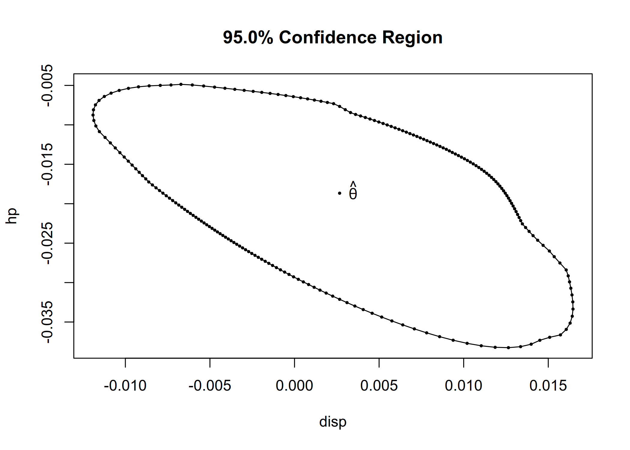
data("clothianidin")
fit2_lm <- el_lm(clo ~ -1 + trt, data = clothianidin)
summary(fit2_lm)
#>
#>  Empirical Likelihood
#>
#> Model: lm
#>
#> Call:
#> el_lm(formula = clo ~ -1 + trt, data = clothianidin)
#>
#> Number of observations: 102
#> Number of parameters: 4
#>
#> Parameter values under the null hypothesis:
#>     trtNaked trtFungicide       trtLow      trtHigh
#>            0            0            0            0
#>
#> Lagrange multipliers:
#> [1] -4.116e+06 -7.329e-01 -1.751e+00 -1.418e-01
#>
#> Maximum EL estimates:
#>     trtNaked trtFungicide       trtLow      trtHigh
#>       -4.479       -3.427       -2.800       -1.307
#>
#> logL: -918.9 , logLR: -447.2
#> Chisq: 894.4, df: 4, Pr(>Chisq): < 2.2e-16
#> EL evaluation: maximum iterations reached
#>
#> Coefficients:
#>              Estimate   Chisq Pr(>Chisq)
#> trtNaked       -4.479 411.072    < 2e-16 ***
#> trtFungicide   -3.427  59.486   1.23e-14 ***
#> trtLow         -2.800  62.955   2.11e-15 ***
#> trtHigh        -1.307   4.653      0.031 *
#> ---
#> Signif. codes:  0 '***' 0.001 '**' 0.01 '*' 0.05 '.' 0.1 ' ' 1
confint(fit2_lm)
#>                  lower      upper
#> trtNaked     -5.002118 -3.9198229
#> trtFungicide -4.109816 -2.6069870
#> trtLow       -3.681837 -1.9031795
#> trtHigh      -2.499165 -0.1157222


## Generalized linear model
data("thiamethoxam")
fit_glm <- el_glm(visit ~ log(mass) + fruit + foliage + var + trt,
  family = quasipoisson(link = "log"), data = thiamethoxam,
  control = el_control(maxit = 100, tol = 1e-08, nthreads = 4)
)
summary(fit_glm)
#>
#>  Empirical Likelihood
#>
#> Model: glm (quasipoisson family with log link)
#>
#> Call:
#> el_glm(formula = visit ~ log(mass) + fruit + foliage + var +
#>     trt, family = quasipoisson(link = "log"), data = thiamethoxam,
#>     control = el_control(maxit = 100, tol = 1e-08, nthreads = 4))
#>
#> Number of observations: 165
#> Number of parameters: 8
#>
#> Parameter values under the null hypothesis:
#> (Intercept)   log(mass)       fruit     foliage       varGZ    trtSpray
#>     -0.1098      0.0000      0.0000      0.0000      0.0000      0.0000
#>   trtFurrow     trtSeed         phi
#>      0.0000      0.0000      1.4623
#>
#> Lagrange multipliers:
#> [1]   1319.19    210.54    -12.99 -24069.07   -318.90   -189.14    -53.35
#> [8]    262.32   -170.21
#>
#> Maximum EL estimates:
#> (Intercept)   log(mass)       fruit     foliage       varGZ    trtSpray
#>    -0.10977     0.24750     0.04654   -19.40632    -0.25760     0.06724
#>   trtFurrow     trtSeed
#>    -0.03634     0.34790
#>
#> logL: -2272 , logLR: -1429
#> Chisq: 2859, df: 7, Pr(>Chisq): < 2.2e-16
#> Constrained EL: initialization failed
#>
#> Coefficients:
#>              Estimate   Chisq Pr(>Chisq)
#> (Intercept)  -0.10977   0.090      0.764
#> log(mass)     0.24750 425.859    < 2e-16 ***
#> fruit         0.04654  29.024   7.15e-08 ***
#> foliage     -19.40632  65.181   6.83e-16 ***
#> varGZ        -0.25760  17.308   3.18e-05 ***
#> trtSpray      0.06724   0.860      0.354
#> trtFurrow    -0.03634   0.217      0.641
#> trtSeed       0.34790  19.271   1.13e-05 ***
#> ---
#> Signif. codes:  0 '***' 0.001 '**' 0.01 '*' 0.05 '.' 0.1 ' ' 1
#>
#> Dispersion for quasipoisson family: 1.462288


## Test of no treatment effect
contrast <- c(
  "trtNaked - trtFungicide", "trtFungicide - trtLow", "trtLow - trtHigh"
)
elt(fit2_lm, lhs = contrast)
#>
#>  Empirical Likelihood Test
#>
#> Hypothesis:
#> trtNaked - trtFungicide = 0
#> trtFungicide - trtLow = 0
#> trtLow - trtHigh = 0
#>
#> Significance level: 0.05, Calibration: Chi-square
#>
#> Statistic: 26.6, Critical value: 7.815
#> p-value: 7.148e-06
#> Constrained EL: converged


## Multiple testing
contrast2 <- rbind(
  c(0, 0, 0, 0, 0, 1, 0, 0),
  c(0, 0, 0, 0, 0, 0, 1, 0),
  c(0, 0, 0, 0, 0, 0, 0, 1)
)
elmt(fit_glm, lhs = contrast2)
#>
#>  Empirical Likelihood Multiple Tests
#>
#> Overall significance level: 0.05
#>
#> Calibration: Multivariate chi-square
#>
#> Hypotheses:
#>               Estimate  Chisq Df
#> trtSpray = 0   0.06724  0.860  1
#> trtFurrow = 0 -0.03634  0.217  1
#> trtSeed = 0    0.34790 19.271  1
Please note that this package is released with a Contributor Code of Conduct. By contributing to this project, you agree to abide by its terms.
These binaries (installable software) and packages are in development.
They may not be fully stable and should be used with caution. We make no claims about them.
Health stats visible at Monitor.