The hardware and bandwidth for this mirror is donated by dogado GmbH, the Webhosting and Full Service-Cloud Provider. Check out our Wordpress Tutorial.
If you wish to report a bug, or if you are interested in having us mirror your free-software or open-source project, please feel free to contact us at mirror[@]dogado.de.

mcstatsim

About

mcstatsim is a lightweight, functional-style toolkit for Monte Carlo simulation studies. Its core is a higher-order driver, runsim(): you write the simulation as a function of its parameters, and runsim() maps it over a grid of conditions, owning the iteration, parallelism, reproducible random-number streams, error capture and result assembly. Around it the package ships ready-to-use performance measures, an evaluation layer that turns raw replicates into a tidy results table, and diagnostic plots.

The only hard dependency is functionals. ggplot2 is used by the plotting helpers and is optional.

How it works

runsim() takes a grid of conditions (one row per scenario), a simulation function whose arguments match the grid columns, and the number of replications. It builds one flat list of n * nrow(grid) jobs, runs them in a single load-balanced parallel pass, and row-binds the results into a data frame with the grid columns, the quantities returned by the simulation function, and a replication index ID.

Installation

install.packages("mcstatsim")                    # released version
# install.packages("remotes")
remotes::install_github("ielbadisy/mcstatsim")   # development version

A complete example

We evaluate the normal-theory 95% confidence interval for a mean when the data are drawn either from a normal distribution or from a skewed (centred log-normal) distribution, across three sample sizes. The true mean is 0 in every cell, so we expect bias near zero and coverage near 0.95, but the t-interval is known to under-cover under skew at small n.

1. Simulation function and grid

library(mcstatsim)

sim_mean_ci <- function(n, dist) {
  x <- if (dist == "normal") rnorm(n) else rlnorm(n) - exp(0.5)  # both have mean 0
  est <- mean(x)
  se  <- sd(x) / sqrt(n)
  crit <- qt(0.975, df = n - 1)
  data.frame(
    est      = est,
    lo       = est - crit * se,
    hi       = est + crit * se,
    true_val = 0
  )
}

grid <- expand.grid(n = c(10, 30, 100), dist = c("normal", "lognormal"),
                    stringsAsFactors = FALSE)
grid
#>     n      dist
#> 1  10    normal
#> 2  30    normal
#> 3 100    normal
#> 4  10 lognormal
#> 5  30 lognormal
#> 6 100 lognormal

2. Run the simulation

seed gives every job its own independent L'Ecuyer-CMRG stream, so the run is reproducible and does not depend on the number of cores.

res <- runsim(
  n           = 2000,
  grid_params = grid,
  sim_func    = sim_mean_ci,
  seed        = 2025,
  num_cores   = 2,
  show_progress = FALSE
)

head(res)
#>     n      dist          est          lo         hi true_val ID
#> 1  10    normal  0.433489939 -0.35003582 1.21701569        0  1
#> 2  30    normal -0.363420104 -0.74905905 0.02221884        0  1
#> 3 100    normal  0.162087539 -0.03781371 0.36198879        0  1
#> 4  10 lognormal  0.292061905 -1.37614955 1.96027336        0  1
#> 5  30 lognormal -0.147570162 -0.56076715 0.26562683        0  1
#> 6 100 lognormal  0.004260512 -0.37423359 0.38275461        0  1
nrow(res)
#> [1] 12000

3. Turn replicates into a performance table

perf <- summarise_sim(
  res,
  by = c("n", "dist"),
  measures = list(
    bias     = ~ calc_bias(est, true_val[1]),
    coverage = ~ calc_coverage(lo, hi, true_val[1]),
    width    = ~ calc_width(lo, hi)
  )
)
perf
#>     n      dist n_sim    bias bias_mcse coverage coverage_mcse  width
#> 1  10 lognormal  2000 -0.0113    0.0153   0.8370        0.0083 2.4341
#> 2  10    normal  2000  0.0092    0.0068   0.9515        0.0048 1.3913
#> 3  30 lognormal  2000 -0.0009    0.0090   0.8750        0.0074 1.4440
#> 4  30    normal  2000  0.0016    0.0042   0.9455        0.0051 0.7402
#> 5 100 lognormal  2000 -0.0007    0.0048   0.9190        0.0061 0.8079
#> 6 100    normal  2000 -0.0004    0.0023   0.9470        0.0050 0.3957
#>   width_mcse
#> 1     0.0396
#> 2     0.0075
#> 3     0.0181
#> 4     0.0022
#> 5     0.0062
#> 6     0.0006

Each calc_* measure contributes its estimate and its Monte Carlo standard error (the *_mcse columns). Numeric columns are rounded to digits (default 4); pass digits = NULL to summarise_sim() for full precision.

4. Diagnostics

Check that no replicate produced a non-finite estimate:

check_estimates(res, by = c("n", "dist"))
#> [1] n        dist     column   n_bad    n_total  prop_bad
#> <0 rows> (or 0-length row.names)

How many replications would we need to pin the coverage MCSE down to 0.0025?

data.frame(perf[c("n", "dist")],
           coverage_mcse = round(perf$coverage_mcse, 4),
           reps_for_0.0025 = mcse_target(perf$coverage_mcse, perf$n_sim, target = 0.0025))
#>     n      dist coverage_mcse reps_for_0.0025
#> 1  10 lognormal        0.0083           22045
#> 2  10    normal        0.0048            7373
#> 3  30 lognormal        0.0074           17524
#> 4  30    normal        0.0051            8324
#> 5 100 lognormal        0.0061           11908
#> 6 100    normal        0.0050            8000

5. Plots

Convergence trace. The running mean of the point estimate with a Monte Carlo standard-error band, one panel per condition:

plot_convergence(res, "est", by = c("n", "dist"))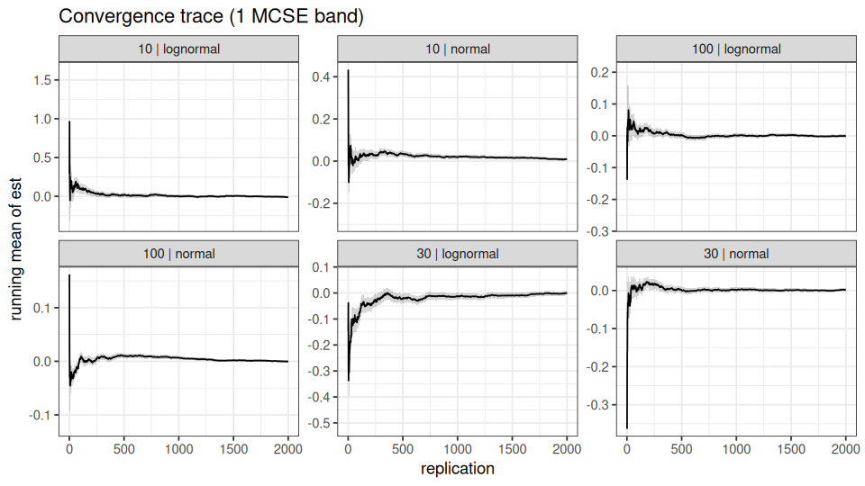

Zip plot (Morris, White and Crowther, 2019). Confidence intervals sorted by the extremeness of their z-statistic and coloured by whether they cover; a well-calibrated interval fills the panel up to the nominal line in the “covers” colour. Shown here for n = 10:

plot_zip(res[res$n == 10, ], "lo", "hi", "true_val", by = "dist")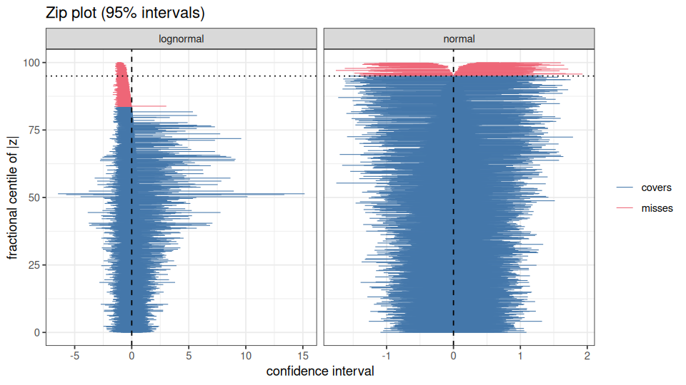

Performance across the design. Coverage with a +/- 2 MCSE bar against the nominal 0.95 line:

plot_performance(perf, "coverage", x = "n", colour = "dist", ref = 0.95)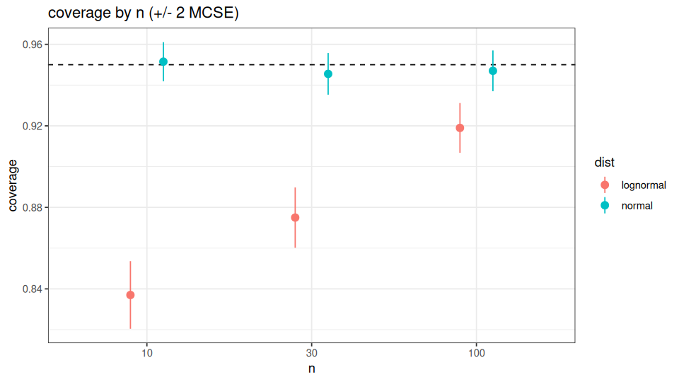

The log-normal intervals under-cover at n = 10 (the zip plot shows the misses concentrated on one side, the signature of skew) and climb back toward 0.95 as n grows. The normal-data intervals sit on 0.95 throughout.

Reproducibility and error handling

a <- runsim(200, grid, sim_mean_ci, seed = 1, num_cores = 1, show_progress = FALSE)
b <- runsim(200, grid, sim_mean_ci, seed = 1, num_cores = 4, show_progress = FALSE)
identical(a$est, b$est)
#> [1] TRUE

If a simulation function errors on some cells, on_error = "warn" (or "omit") drops those jobs and records them in attr(x, "errors"), which failure_summary() aggregates per condition. Warnings raised inside the simulation function are kept in attr(x, "warnings").

fragile <- function(n, dist) {
  if (dist == "lognormal" && n == 10 && runif(1) < 0.1) stop("fit did not converge")
  sim_mean_ci(n, dist)
}
r <- runsim(200, grid, fragile, seed = 1, on_error = "omit",
            num_cores = 1, show_progress = FALSE)
nrow(r)
#> [1] 1179
failure_summary(r)
#>    n      dist n_failed failure_rate        example_error
#> 1 10 lognormal       21        0.105 fit did not converge

A save_path makes a long run resumable: the result is checkpointed after each chunk of checkpoint_every replications, and re-running runsim() with the same save_path, n, grid_params and seed loads the completed replications and runs only the rest. A resumed run reproduces an uninterrupted one exactly.

ckpt <- tempfile(fileext = ".rds")
r1 <- runsim(200, grid, sim_mean_ci, seed = 1, save_path = ckpt,
             checkpoint_every = 50, num_cores = 1, show_progress = FALSE)
identical(r1$est, a$est)
#> [1] TRUE

Performance measures

calc_bias(), calc_variance(), calc_mse(), calc_rmse(), calc_coverage(), calc_width(), calc_rejection_rate(), calc_relative_bias(), calc_relative_mse(), calc_relative_rmse(). Each returns the estimate together with its Monte Carlo standard error, rounded to digits (default 4; NULL for full precision). They can be used on their own or inside summarise_sim().

est <- res$est[res$n == 30 & res$dist == "normal"]
calc_bias(est, 0)
#> $bias
#> [1] 0.0016
#> 
#> $bias_mcse
#> [1] 0.0042
calc_rmse(est, 0, digits = NULL)
#> $rmse
#> [1] 0.1860117
#> 
#> $rmse_mcse
#> [1] 0.003563415

Lower-level helpers

mcpmap() maps a function over equal-length named lists in parallel (via functionals), and combine_df() row-binds a list of lists of data frames, adding a source ID. runsim() covers most use cases; these are there for custom drivers.

mcpmap(list(a = 1:3, b = 4:6), function(a, b) a + b, num_cores = 1,
       show_progress = FALSE)
#> [[1]]
#> [1] 5
#> 
#> [[2]]
#> [1] 7
#> 
#> [[3]]
#> [1] 9

Features

• Higher-order, declarative interface: write the simulation as a function; runsim() maps it over the design.
• Reproducible parallelism: per-job RNG streams; results independent of core count.
• Robustness: per-cell error/warning capture, checkpoint/resume for long runs.
• Evaluation layer: summarise_sim() plus a full set of MCSE-aware measures.
• Diagnostics: convergence traces, zip plots, performance plots, non-finite checks.

Learn more

The package vignette, “Monte Carlo simulation studies with mcstatsim” (PDF), walks through runsim(), reproducible RNG, error handling, checkpoint/resume, summarise_sim(), the calc_* measures, diagnostics and plots, with a worked case study:

vignette("mcstatsim", package = "mcstatsim")

Citation

To cite mcstatsim in publications, use:

citation("mcstatsim")
#> To cite mcstatsim in publications, use:
#> 
#>   El Badisy I (2026). _mcstatsim: Monte Carlo Statistical Simulation
#>   Tools Using a Functional Approach_. R package version 0.9.2,
#>   <https://CRAN.R-project.org/package=mcstatsim>.
#> 
#> A BibTeX entry for LaTeX users is
#> 
#>   @Manual{,
#>     title = {mcstatsim: Monte Carlo Statistical Simulation Tools Using a Functional Approach},
#>     author = {Imad {El Badisy}},
#>     year = {2026},
#>     note = {R package version 0.9.2},
#>     url = {https://CRAN.R-project.org/package=mcstatsim},
#>   }

Contributing

Contributions are welcome. Please feel free to open an issue or submit a pull request.

These binaries (installable software) and packages are in development.
They may not be fully stable and should be used with caution. We make no claims about them.
Health stats visible at Monitor.