README

The hardware and bandwidth for this mirror is donated by dogado GmbH, the Webhosting and Full Service-Cloud Provider. Check out our Wordpress Tutorial.
If you wish to report a bug, or if you are interested in having us mirror your free-software or open-source project, please feel free to contact us at mirror[@]dogado.de.

matSPACE

This is a README file of the R package matSPACE. Our package fits sparse partial correlation networks for matrix-variate data, i.e. observations that are themselves p x q matrices rather than a single vector of q measurements. We extend the SPACE (Sparse PArtial Correlation Estimation) joint estimation framework to a Kronecker-product precision structure, Omega = V %x% U, where V (q x q) is the column-wise precision matrix and U (p x p) is the row-wise precision matrix. All partial correlations are estimated jointly via an L1-penalized (lasso) shooting algorithm, which preserves symmetry of the estimated network and avoids the tuning-parameter selection difficulties of separate node-wise regressions.

Installation of the package

install.packages("matSPACE")

# development version
# install.packages("pak")
pak::pak("kimhyew1/matSPACE")

A basic example of using the package

We give a toy example to apply the main function matSPACE, which estimates the Kronecker-structured row/column precision matrices U and V.

Generate data

We first generate simulated matrix-variate data. Columns 1-2 and columns 3-4 are correlated by construction, so there is real sparse structure for matSPACE to recover (pure noise data has no structure to penalize away, so the BIC-optimal fit is always the fully sparse one).

set.seed(1)
p = 5
q = 4
n = 20

library(matSPACE)
data = replicate(n, {
  mat = matrix(rnorm(p * q), p, q)
  mat[, 2] = mat[, 2] + 0.8 * mat[, 1]
  mat[, 4] = mat[, 4] + 0.8 * mat[, 3]
  mat
}, simplify = FALSE)

Model fitting

Applying matSPACE to the simulated data, a lasso penalty path is searched for V and U separately, and the BIC-minimizing fit is returned for each.

fit = matSPACE(data, K = 10)
fit$V   # q x q column-wise precision matrix
#>             [,1]        [,2]        [,3]        [,4]
#> [1,]  1.00000000 -0.48986779  0.00000000 -0.09720007
#> [2,] -0.48986779  0.67543509 -0.05648484  0.00000000
#> [3,]  0.00000000 -0.05648484  1.03329539 -0.48039780
#> [4,] -0.09720007  0.00000000 -0.48039780  0.82809375
fit$U   # p x p row-wise precision matrix
#>            [,1]       [,2]        [,3]      [,4]        [,5]
#> [1,]  1.2461467 0.19063125 -0.30984454 0.0000000 -0.16769017
#> [2,]  0.1906313 1.52167139  0.00000000 0.1972048  0.07992512
#> [3,] -0.3098445 0.00000000  1.78285206 0.0000000 -0.09210015
#> [4,]  0.0000000 0.19720479  0.00000000 1.3713710  0.12289066
#> [5,] -0.1676902 0.07992512 -0.09210015 0.1228907  1.56699009

Visualization of the lambda path

The full lambda path behind this selection is attached as a "path" attribute, which lets us plot BIC against lambda without refitting.

path = attr(fit, "path")
plot(log(path$V$lambda), path$V$bic, type = "b",
     xlab = "log(lambda)", ylab = "BIC", main = "Column (V) lambda path")
i_min = which.min(path$V$bic)
points(log(path$V$lambda[i_min]), path$V$bic[i_min], col = "red", pch = 19)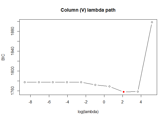

Fitting with a single lasso penalty

If you already know the penalty you want, space fits a single lasso penalty directly, without searching a path.

fit_single = space(data, lam = 0.5)
fit_single$ParCor
#>           [,1]       [,2]       [,3]       [,4]
#> [1,] 1.0000000 0.62797406 0.00000000 0.13888124
#> [2,] 0.6279741 1.00000000 0.09220064 0.06565944
#> [3,] 0.0000000 0.09220064 1.00000000 0.55404153
#> [4,] 0.1388812 0.06565944 0.55404153 1.00000000

Issues

These binaries (installable software) and packages are in development.
They may not be fully stable and should be used with caution. We make no claims about them.
Health stats visible at Monitor.