install.packages("mapboxapi")
# For the development version:
# remotes::install_github("walkerke/mapboxapi")

# Get your access token from your Mapbox account and save it in R; save a public token, 
# secret token, or both with successive calls to mb_access_token()
mapboxapi::mb_access_token("pk.eyzdl....", install = TRUE)

library(shiny)
library(mapdeck)
library(mapboxapi)

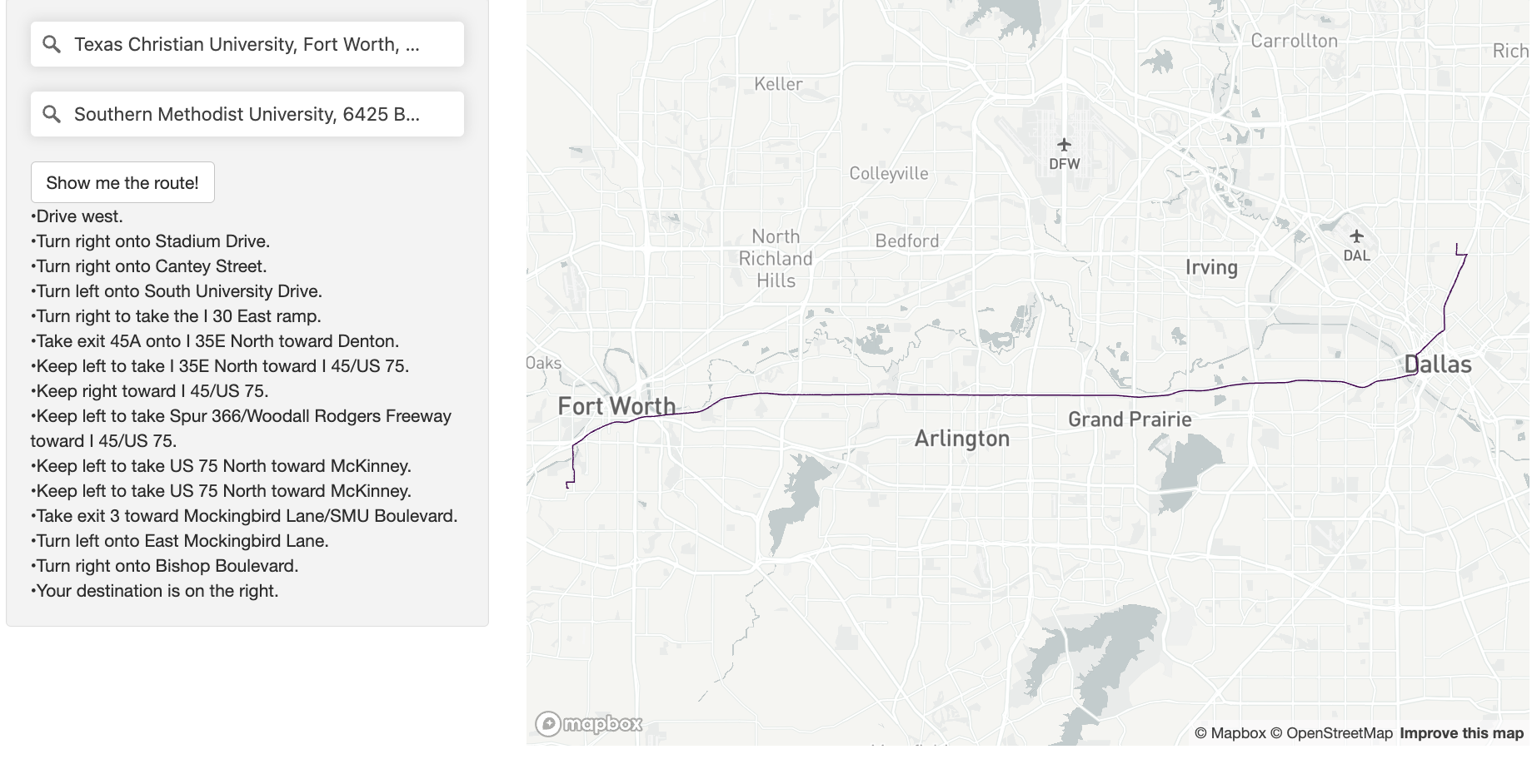
# Set up a sidebar panel with geocoders for origin and destination,
# and a placeholder to print out the driving instructions
ui <- fluidPage(
  tags$head(
    tags$style(HTML(
      "#origin {
        position: relative;
        z-index: 999999;    
      }"
    ))
  ),
  sidebarPanel(
    mapboxGeocoderInput("origin", placeholder = "Enter an origin",
                        proximity = mb_geocode("Fort Worth, TX")),
    shiny::br(),
    mapboxGeocoderInput("destination", placeholder = "Enter a destination",
                        proximity = mb_geocode("Fort Worth, TX")),
    shiny::br(),
    actionButton("action", "Show me the route!"),
    htmlOutput("instructions"),
    width = 4
  ),
  mainPanel(
    mapdeckOutput(outputId = "map", width = "100%", height = 600)
  )
)

# Set up reactive elements to generate routes when the action button is clicked,
# then map the routes and print out the driving directions
server <- function(input, output) {

  output$map <- renderMapdeck({
    mapdeck(token = Sys.getenv("MAPBOX_PUBLIC_TOKEN"),
            style = mapdeck_style("light"),
            zoom = 11,
            location = c(-97.3034314, 32.7593745))

  })

  new_route <- eventReactive(input$action, {
    mb_directions(
      input_data = rbind(
        geocoder_as_sf(input$origin),
        geocoder_as_sf(input$destination)
      ),
      profile = "driving",
      output = "sf",
      steps = TRUE
    )
  })

  observeEvent(new_route(), {

    mapdeck_update(map_id = "map") %>%
      clear_path(layer_id = "new_route") %>%
      add_path(data = new_route(), stroke_width = 75,
               layer_id = "new_route", update_view = TRUE,
               focus_layer = TRUE)

    output$instructions <- renderUI({
      HTML(paste0(
        paste("&bull;", new_route()$instruction, sep = ""),
        collapse = "<br/>"))
    })
  })

}

shinyApp(ui = ui, server = server)

library(mapboxapi)
library(mapdeck)
library(httr)

# Get the Microsoft buildings data for Texas and unzip
GET("https://usbuildingdata.blob.core.windows.net/usbuildings-v1-1/Texas.zip",
    write_disk("Texas.zip", overwrite = TRUE), progress())

unzip("Texas.zip")

# Use tippecanoe to make a dynamic .mbtiles file that visualizes large data appropriately
# at any zoom level.  sf objects can also be used as input!
# (requires installing tippecanoe on your machine separately first)
tippecanoe(input = "Texas.geojson",
           output = "Texas.mbtiles",
           layer_name = "texas_buildings")

# Upload the generated tileset to your Mapbox account (requires a Mapbox secret access token
# to be set as an environment variable)
upload_tiles(input = "Texas.mbtiles", username = "kwalkertcu",
             tileset_id = "TX_buildings",
             multipart = TRUE)


# Head over to Mapbox Studio when the upload is done (check the status with
# `check_upload_status()`) and add it to a style.  When you've styled it, bring it back
# into R with mapdeck by referencing the style ID:
mapdeck(token = Sys.getenv("MAPBOX_PUBLIC_TOKEN"),
        style = "mapbox://styles/kwalkertcu/ckaf9qxim1pyk1io7r2e8exj2/draft",
        zoom = 6,
        location = c(-98.7382803, 31.7678448))

library(mapboxapi)
library(tidyverse)
library(tidycensus)
library(tigris)
library(sf)
library(crsuggest)
options(tigris_use_cache = TRUE)

# Grab median gross rent data from the  ACS for the Twin Cities metro
county_names <- c("Hennepin", "Ramsey", "Anoka", "Washington",
                  "Dakota", "Carver", "Scott")

tc_rent <- get_acs(geography = "tract",
                   variables = "B25064_001",
                   state = "MN",
                   county = county_names,
                   year = 2022,
                   geometry = TRUE)

# Find the right coordinate system to use; in this case we'll use 26993
print(suggest_top_crs(tc_rent, units = "m"))

# Remove water areas - there are a lot in Minnesota! - to help ensure that a point in a 
# given Census tract will be routable
tc_rent_points <- tc_rent %>%
  st_transform(26993) %>%
  erase_water(area_threshold = 0.95) %>%
  st_point_on_surface()

# Determine the location of downtown (apologies to St. Paul, purposes of illustration here)
downtown_mpls <- mb_geocode("Minneapolis City Hall, Minneapolis MN")

# Use mb_matrix() to calculate driving time from all Twin Cities Census tracts to downtown
time_to_downtown <- mb_matrix(origins = tc_rent_points,
                              destinations = downtown_mpls) %>%
  as.vector()

tc_rent$time <- time_to_downtown

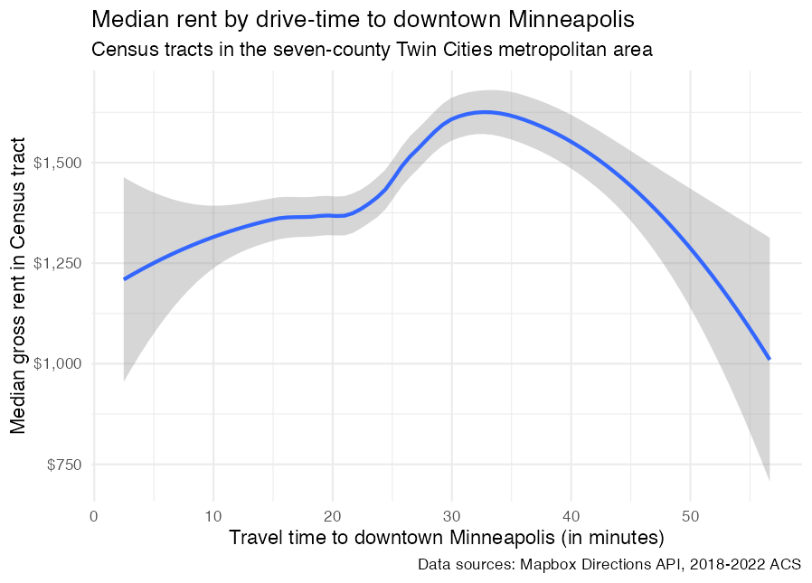
# Visualize how rent varies by travel time from downtown with ggplot2
ggplot(tc_rent, aes(x = time, y = estimate)) +
  geom_smooth() +
  scale_y_continuous(labels = scales::dollar) +
  labs(x = "Travel time to downtown Minneapolis (in minutes)",
       y = "Median gross rent in Census tract", 
       title = "Median rent by drive-time to downtown Minneapolis",
       subtitle = "Census tracts in the seven-county Twin Cities metropolitan area",
       caption = "Data sources: Mapbox Directions API, 2018-2022 ACS") + 
  theme_minimal()