The hardware and bandwidth for this mirror is donated by dogado GmbH, the Webhosting and Full Service-Cloud Provider. Check out our Wordpress Tutorial.
If you wish to report a bug, or if you are interested in having us mirror your free-software or open-source project, please feel free to contact us at mirror[@]dogado.de.
![]()
macroBiome is an R package that provides functions with both point and grid modes for simulating biomes by equilibrium vegetation models, with a special focus on paleoenvironmental applications.
Three widely used equilibrium biome models are currently implemented in the package: the Holdridge Life Zone (HLZ) system (Holdridge 1947), the Köppen-Geiger classification (KGC) system (Köppen 1936) and the BIOME model (Prentice et al. 1992). Three climatic forest-steppe models are also implemented.
An approach for estimating monthly time series of relative sunshine duration from temperature and precipitation data (Yin 1999) is also adapted, allowing process-based biome models to be combined with high-resolution paleoclimate simulation datasets (e.g., CHELSA-TraCE21k v1.0 dataset).
Installing the latest stable version from CRAN:
install.packages("macroBiome")You can install the development version of macroBiome like so:
if (!require(devtools)) install.packages("devtools")
devtools::install_github("szelepcsenyi/macroBiome")Create a biome map of the Eastern Mediterranean–Black Sea–Caspian-Corridor region for the period 1991-2020 using the CRU TS v.4.05 dataset (Harris et al. 2020)
list.of.packages <- c("R.utils", "rasterVis", "latticeExtra", "rnaturalearth")
new.packages <- list.of.packages[!(list.of.packages %in% installed.packages()[,"Package"])]
if (length(new.packages)) { install.packages(new.packages) }

library(macroBiome)
library(terra)
library(raster)
library(rasterVis)

# Target domain: Eastern Mediterranean–Black Sea–Caspian-Corridor region
e <- raster(crs = "+proj=longlat +datum=WGS84 +no_defs",
            ext = extent(20., 60., 33., 49.),
            resolution = 0.5)

# Set some magic numbers and parameters
fiyr <- 1991
n_moy <- 12
n_dec <- 3
l_dec <- 10
path <- "https://crudata.uea.ac.uk/cru/data/hrg/cru_ts_4.05/cruts.2103051243.v4.05/"
cv.var_lbl <- c("tmp", "pre", "cld")
cv.ts <- paste0(seq(fiyr, by = l_dec, length.out = n_dec), ".",
                seq(fiyr + l_dec - 1, by = l_dec, length.out = n_dec), ".")

# Download the annual time series of meteorological data, and
# compute their multi-year averages
for (i_var in 1 : length(cv.var_lbl)) {
  rstr <- raster::stack()
  for (i_ts in 1 : length(cv.ts)) {
    fileLCL <- tempfile(fileext = ".nc.gz")
    fileRMT <- paste0(path, cv.var_lbl[i_var], "/cru_ts4.05.",
                      cv.ts[i_ts], cv.var_lbl[i_var], ".dat.nc.gz")
    download.file(fileRMT, destfile = fileLCL, mode = "wb")
    nc <- R.utils::gunzip(fileLCL)
    rstr <- stack(rstr, crop(brick(nc, varname = cv.var_lbl[i_var]), e))
  }
  rstr <- stackApply(rstr, indices = rep(seq(1, n_moy), (n_dec * l_dec)),
                     fun = mean, na.rm = FALSE)
  assign(cv.var_lbl[i_var], round(rstr, 1))
  rm(rstr)
}

# Convert cloudiness values to relative sunshine duration data
# For the approach used, see Doorenbos and Pruitt (1977)
# https://www.fao.org/3/f2430e/f2430e.pdf
bsd <- calc(cld, fun = macroBiome:::cldn2bsdf)

# Download the altitude data (use the TBASE data)
url <- "http://research.jisao.washington.edu/data_sets/elevation/elev.0.5-deg.nc"
tmpy <- tempfile()
download.file(url, tmpy, mode = "wb")
elv <- stack(tmpy)
elv <- crop(rotate(elv), e)
elv[elv < 0.] <- 0.

# Apply the BIOME model
year <- trunc(mean(seq(fiyr, fiyr + (n_dec * l_dec) - 1)))
rs.BIOME <- cliBIOMEGrid(tmp, pre, bsd, elv, sc.year = year)

# Make a color key for vegetation classes used in the BIOME model
Name <- vegClsNumCodes$Code.BIOME[!is.na(vegClsNumCodes$Code.BIOME)]
Col <- c("#01665E", "#5AB4AC", "#8C510A", "#FB9A99", "#64D264", "#C9FFC9",
         "#147814", "#6A3D9A", "#22E6FF", "#0000E7", "#E31A1C", "#D8B365",
         "#F6E8C3", "#CAB2D6", "#FF7F00", "#FDBF6F", "#D1E5F0")
bioColours <- data.frame(Code = seq(1, length(Name)), Name = Name, Col = Col)
rm(Name, Col)

# Reclassify the raw data of the generated biome map
slctd <- as.numeric(levels(factor(values(rs.BIOME)[!is.na(values(rs.BIOME))])))
reclass_mtx <- matrix(c(NA, slctd, NA, seq(1, length(slctd))), ncol = 2)
biome <- as.factor(classify(rs.BIOME, reclass_mtx))
class <- unlist(lapply(reclass_mtx[-1, 1],
                       function(i) { subset(bioColours, Code == i, select = Name)}))
rat <- data.frame(ID = reclass_mtx[-1, 2], class = class)
levels(biome)[[1]] <- rat

# Plot the biome map
main <- "Eastern Mediterranean–Black Sea–Caspian-Corridor region"
plt <- levelplot(biome, main = main, col.regions = bioColours$Col[slctd],
                 colorkey = list(space = "bottom", height = 1.1), pretty = T,
                 par.settings = list(layout.widths = list(axis.key.padding = 4)))
plt <- plt + latticeExtra::layer(sp.lines(as(rnaturalearth::countries110, "Spatial"),
                                          col = "gray30", lwd = 2.0))
print(plt)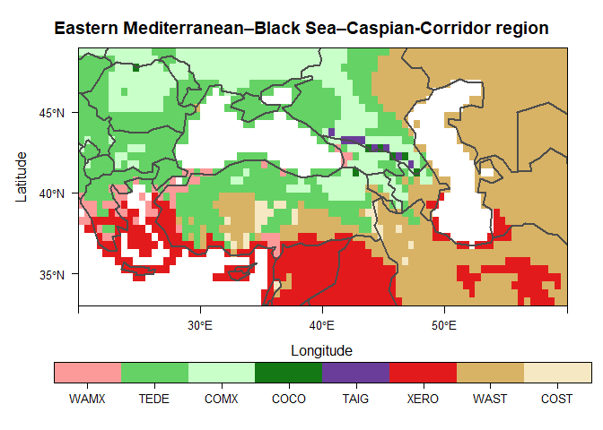
citation("macroBiome")To cite package ‘macroBiome’ in publications use:
Szelepcsényi Z (2024) macroBiome: A Tool for Mapping the Distribution of the Biomes and Bioclimate. R package version 0.4.0. https://doi.org/10.5281/zenodo.7633367
I have invested a considerable amount of time and effort in creating the package ‘macroBiome’. Please cite it if you use it.
These binaries (installable software) and packages are in development.
They may not be fully stable and should be used with caution. We make no claims about them.
Health stats visible at Monitor.