The hardware and bandwidth for this mirror is donated by dogado GmbH, the Webhosting and Full Service-Cloud Provider. Check out our Wordpress Tutorial.
If you wish to report a bug, or if you are interested in having us mirror your free-software or open-source project, please feel free to contact us at mirror[@]dogado.de.

lwpls

lwpls implements locally-weighted partial least squares (LW-PLS) for the tidymodels ecosystem.

LW-PLS is a just-in-time learning method used in chemometrics and process monitoring (soft sensors). Instead of fitting a single global model, it builds a dedicated weighted PLS model around each new sample, where every training sample is weighted by its similarity to that sample. A linear method can therefore capture nonlinear and time-varying relationships.

Features

• lwpls(): a parsnip model for regression (one or more outcomes) and classification (LW-PLS-DA).
• Two similarity indexes: the Euclidean distance of the original LW-PLS, and the covariance-based index of CbLW-PLS (similarity = "covariance").
• Robust local models, by partial robust M-regression (set_engine("lwpls", robust = TRUE)), and sparse local models that select their own predictors (sparsity), with the trimmed_rmse() metric to tune robust models on contaminated data.
• A native implementation, validated against Kaneko’s reference implementation, with the prediction kernel written in C++ (RcppArmadillo). Queries are processed in blocks, so most of the work runs as BLAS matrix-matrix products.
• Tuning with tune and dials: localization() and similarity() are tuning parameters, and all values of num_comp are evaluated from a single fit (the “submodel trick”).
• lwpls_fit(): a standalone hardhat modeling function with matrix, data frame, formula and recipe interfaces.
• Diagnostics for spectroscopy (lwpls_local()) with publication-ready ggplot2 plots: reliability of each prediction (applicability domain), local regression vectors along the spectrum, robust weights that point to wrong reference values, and wavelengths selected by sparse models.

Installation

Install a prebuilt binary from r-universe, which needs no compiler:

install.packages(
  "lwpls",
  repos = c("https://christiangoueguel.r-universe.dev", "https://cloud.r-project.org")
)

Or build the development version from GitHub with:

# install.packages("pak")
pak::pak("ChristianGoueguel/lwpls")

Building from source compiles C++ code, so it needs the R compiler tools. On macOS, that includes gfortran from https://mac.r-project.org/tools/.

Example

Predict the water content of meat samples from their near-infrared spectra and tune both hyperparameters with cross-validation:

library(tidymodels)
library(lwpls)

data(meats, package = "modeldata")
meats <- meats |> select(-fat, -protein)

set.seed(123)
meats_split <- initial_split(meats, prop = 0.75)
meats_folds <- vfold_cv(training(meats_split), v = 5)

lwpls_wflow <- workflow(
  water ~ .,
  lwpls(
    num_comp = tune(), 
    localization = tune()
  ) |> 
    set_mode("regression")
)

lwpls_grid <- grid_regular(
  num_comp(c(1, 15)),
  localization(),
  levels = c(num_comp = 15, localization = 8)
)

lwpls_res <- tune_grid(lwpls_wflow, meats_folds, grid = lwpls_grid)

show_best(lwpls_res, metric = "rmse", n = 3)
#> # A tibble: 3 × 8
#>   num_comp localization .metric .estimator  mean     n std_err .config          
#>      <int>        <dbl> <chr>   <chr>      <dbl> <int>   <dbl> <chr>            
#> 1       10          0.5 rmse    standard    1.66     5   0.156 pre0_mod077_post0
#> 2       13          0.5 rmse    standard    1.68     5   0.198 pre0_mod101_post0
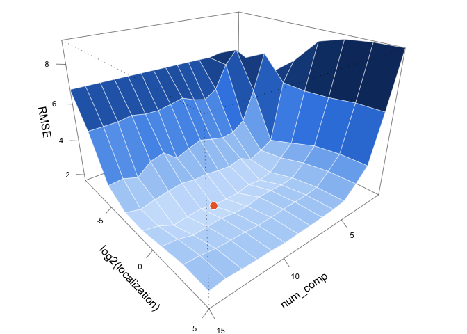
#> 3        9          0.5 rmse    standard    1.70     5   0.174 pre0_mod069_post0

The 120 candidate models are evaluated with only 8 fits per resample. Their cross-validated RMSE forms a surface over the two hyperparameters, with a valley between very local models and global PLS (the best model is the orange point):

rmse_grid <- lwpls_res |>
  collect_metrics() |>
  filter(.metric == "rmse") |>
  select(num_comp, localization, rmse = mean)
best <- slice_min(rmse_grid, rmse)

# color each facet by its mean RMSE
rmse_mat <- with(rmse_grid, tapply(rmse, list(num_comp, log2(localization)), mean))
n <- dim(rmse_mat)
facets <- (rmse_mat[-1, -1] + rmse_mat[-1, -n[2]] + rmse_mat[-n[1], -1] + rmse_mat[-n[1], -n[2]]) / 4
blues <- colorRampPalette(c("#cde2fb", "#3987e5", "#0d366b"))(50)

par(mar = c(1, 0, 0, 0))
view <- persp(
  x = as.numeric(rownames(rmse_mat)), 
  y = as.numeric(colnames(rmse_mat)),
  z = rmse_mat, 
  theta = 140, 
  phi = 25, 
  expand = 0.7, 
  ticktype = "detailed",
  col = blues[cut(facets, 50)], 
  border = "white", 
  lwd = 0.5,
  xlab = "num_comp", 
  ylab = "log2(localization)", 
  zlab = "RMSE", cex.axis = 0.7
)
points(
  trans3d(best$num_comp, log2(best$localization), best$rmse, view), 
  pch = 21, 
  bg = "#eb6834", 
  col = "white", 
  cex = 1.6
)

The final model is evaluated on the test set:

lwpls_wflow |>
  finalize_workflow(select_best(lwpls_res, metric = "rmse")) |>
  last_fit(meats_split) |>
  collect_metrics()
#> # A tibble: 2 × 4
#>   .metric .estimator .estimate .config        
#>   <chr>   <chr>          <dbl> <chr>          
#> 1 rmse    standard       1.38  pre0_mod0_post0
#> 2 rsq     standard       0.978 pre0_mod0_post0

Each prediction comes from its own local model. lwpls_local() returns these models with their diagnostics; for example, their regression vectors along the spectrum (100 channels between 850 and 1050 nm) show how the bands used change with the water content:

final_fit <- lwpls_wflow |>
  finalize_workflow(select_best(lwpls_res, metric = "rmse")) |>
  fit(training(meats_split))

final_fit |>
  lwpls_local(testing(meats_split), wavelength = seq(850, 1050, length.out = 100)) |>
  plot_coefficients(axis_label = "Wavelength (nm)")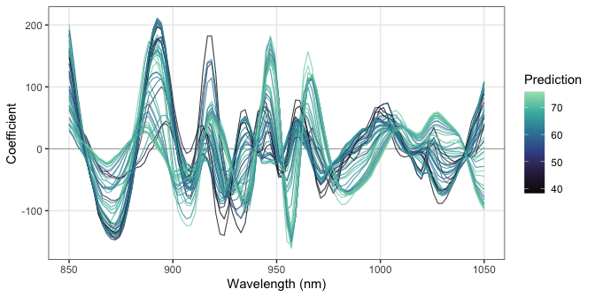

See vignette("lwpls") for more details, including the comparison with global PLS and classification, vignette("robust-sparse") for robust and sparse local models, and vignette("diagnostics") for the diagnostic plots.

How it works

For a query sample \(x_q\), each training sample \(x_i\) receives the weight

\[\omega_i = \exp\left(-\frac{\lVert x_i - x_q \rVert}{\sigma_d \varphi}\right)\]

where \(\sigma_d\) is the standard deviation of the distances and \(\varphi\) is the localization parameter. A PLS model with num_comp components is then fitted with these weights, and the query is projected onto it. Small values of \(\varphi\) give very local models; large values give global PLS.

References

• Kim, S., Kano, M., Nakagawa, H. and Hasebe, S. (2011). Estimation of active pharmaceutical ingredients content using locally weighted partial least squares and statistical wavelength selection. International Journal of Pharmaceutics, 421(2), 269–274. doi:10.1016/j.ijpharm.2011.10.007
• Bevilacqua, M. and Marini, F. (2014). Local classification: Locally weighted-partial least squares-discriminant analysis (LW-PLS-DA). Analytica Chimica Acta, 838, 20–30. doi:10.1016/j.aca.2014.05.057
• Hazama, K. and Kano, M. (2015). Covariance-based locally weighted partial least squares for high-performance adaptive modeling. Chemometrics and Intelligent Laboratory Systems, 146, 55–62. doi:10.1016/j.chemolab.2015.05.007
• Serneels, S., Croux, C., Filzmoser, P. and Van Espen, P. J. (2005). Partial robust M-regression. Chemometrics and Intelligent Laboratory Systems, 79(1–2), 55–64. doi:10.1016/j.chemolab.2005.04.007
• Hoffmann, I., Serneels, S., Filzmoser, P. and Croux, C. (2015). Sparse partial robust M regression. Chemometrics and Intelligent Laboratory Systems, 149, 50–59. doi:10.1016/j.chemolab.2015.09.019
• Lesnoff, M., Metz, M. and Roger, J.-M. (2020). Comparison of locally weighted PLS strategies for regression and discrimination on agronomic NIR data. Journal of Chemometrics, 34(5), e3209. doi:10.1002/cem.3209

These binaries (installable software) and packages are in development.
They may not be fully stable and should be used with caution. We make no claims about them.
Health stats visible at Monitor.