The hardware and bandwidth for this mirror is donated by dogado GmbH, the Webhosting and Full Service-Cloud Provider. Check out our Wordpress Tutorial.
If you wish to report a bug, or if you are interested in having us mirror your free-software or open-source project, please feel free to contact us at mirror[@]dogado.de.

Download and analyse nighttime lights satellite data from R.
lightson supports two data sources:
The ISRO Bhuvan NTL source does not require any authentication. VIIRS requires a free NASA Earthdata account.
pak::pak("saketlab/lightson")library(lightson)
df <- bhuvan_stats() # all states, 2012-2024
head(df)
#> state year mean_radiance
#> 1 Andhra Pradesh 2012 22.4
bihar <- bhuvan_stats(state = "BIHAR")
plot_ntl_trend(bihar, region = "Bihar", caption = "Source: ISRO Bhuvan")states <- c("Bihar", "Maharashtra", "Tamil Nadu", "Uttar Pradesh", "Kerala")
plot_ntl_trend(
df[df$state %in% states, ],
region = states,
subtitle = "Bhuvan state mean radiance (nW/cm^2/sr)",
caption = "Source: ISRO Bhuvan NTL portal"
)library(sf)
library(terra)
states_sf <- get_india_admin("state") # bundled LGD/SoI boundaries, full J&K
rasters <- bhuvan_raster("IND", years = 2022, bbox_pad = c(0, 0, 0, 3.5))
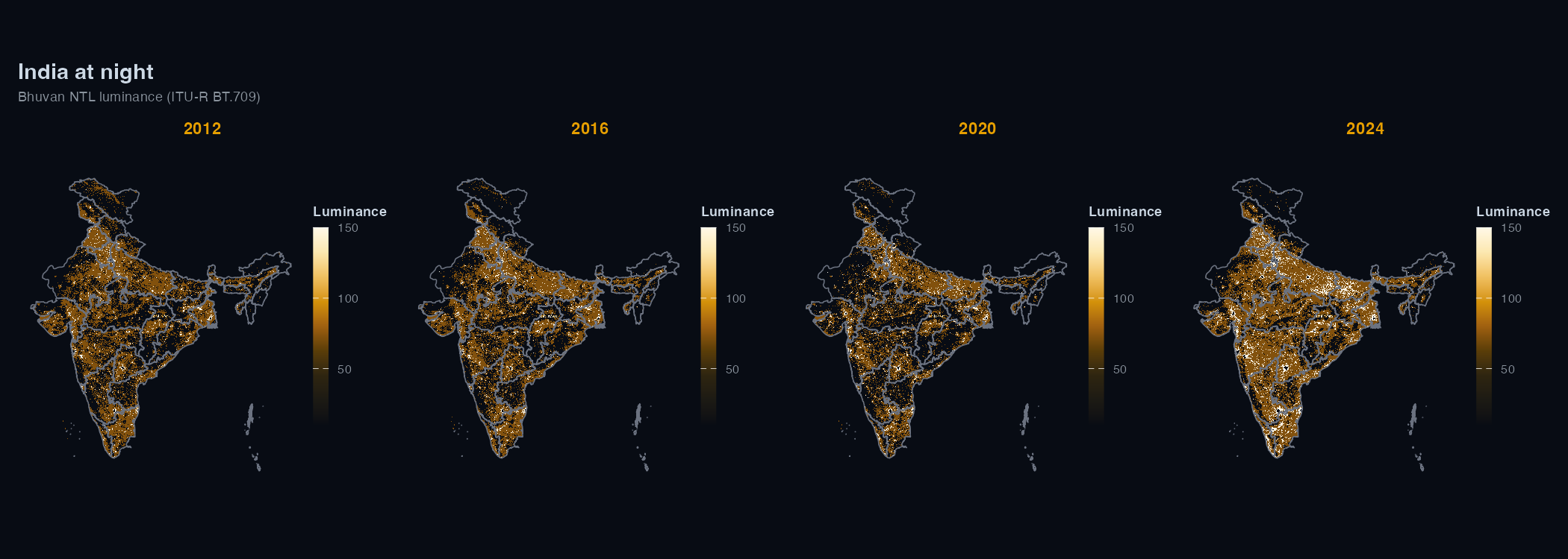
plot_ntl_map(rasters[["2022"]], polygons = states_sf, dark = TRUE)
plot_ntl_map(rasters[["2022"]], polygons = states_sf, palette = "bhuvan")districts <- sf::read_sf("https://bharatviz.org/India-bhuvan-districts.geojson")
rasters <- bhuvan_raster(districts, years = 2018:2023)
panel <- extract_panel(rasters, districts, id_col = "district_name")
head(panel)
#> region_id year mean_radiance n_pixels
#> 1 Adilabad 2018 14.2 3821
plot_ntl_trend(panel, region = c("Mumbai", "Delhi", "Chennai", "Bengaluru"))bhuvan_raster() accepts any sf object
(including your own shapefile/geojson).
VIIRS gives physical radiance in nW/cm^2/sr, which is useful when you need calibrated values or coverage outside India.
Getting a token:
EDL-...
string~/.Renviron:
EARTHDATA_TOKEN=EDL-xxxxxxxxxxxxxxxxxxxx# read EARTHDATA_TOKEN from environment
token <- earthdata_token()
rasters <- ntl_download(region = "IND", years = 2020:2025, token = token)
# Monthly and near-current daily Black Marble
monthly <- ntl_download("IND", 2025, token, product = "monthly")
daily <- ntl_download("IND", token = token, product = "daily",
dates = as.Date("2025-11-12"))
panel <- extract_panel(rasters, get_india_admin("state"), id_col = "state_name")
plot_ntl_trend(panel, region = c("Bihar", "Maharashtra"))You can also set EARTHDATA_USERNAME and
EARTHDATA_PASSWORD in ~/.Renviron instead and
earthdata_token() will fetch the token for you.
Bhuvan WMS rasters are classed maps with four colours (< 5, 5-25,
26-200 and > 200 nW/cm^2/sr). bhuvan_raster() converts
each class to a representative radiance: the midpoints 2.5, 15 and
112.5, and 200 (the floor) for the open-ended top class. These are
banded values, so the brightest areas are underestimated. Use VIIRS when
you need continuous calibrated radiance, and don’t pool the two sources
in a regression without normalising first.
Bhuvan NTL data from 2024 onwards uses VNP46A4 Collection 2.0;
2012-2023 uses Collection 1.0. The two collections use different
calibration algorithms, so estimates aren’t directly comparable across
that boundary. lightson warns automatically when a request
spans both.
These binaries (installable software) and packages are in development.
They may not be fully stable and should be used with caution. We make no claims about them.
Health stats visible at Monitor.