
The hardware and bandwidth for this mirror is donated by dogado GmbH, the Webhosting and Full Service-Cloud Provider. Check out our Wordpress Tutorial.
If you wish to report a bug, or if you are interested in having us mirror your free-software or open-source project, please feel free to contact us at mirror[@]dogado.de.


Calculate and extract remote sensing metrics for spatial health analysis 🛰️. This package offers R users a quick and easy way to obtain areal or zonal statistics of key indicators and covariates, ideal for modeling infectious diseases 🦠 within the framework of spatial epidemiology 🏥.
You can install the development version with:
# install.packages("pak")
pak::pak("harmonize-tools/land4health")library(land4health)
# l4h_install()#> ── rgee 1.1.8 ──────────────────────────────────────── earthengine-api 1.7.38 ──
#> ✔ user: antony.barja8@gmail.com
#> ✔ Initializing Google Earth Engine: ✔ Initializing Google Earth Engine: DONE!
#> ✔ Earth Engine account: projects/1009866941441/assets/BM_Castropampa
#> ✔ Python Path: C:/Python314/python.exe
#> ────────────────────────────────────────────────────────────────────────────────l4h_list_metrics()
#> # A tibble: 10 × 11
#> category metric pixel_resolution_met…¹ dataset start_year end_year
#> <chr> <chr> <chr> <chr> <int> <int>
#> 1 Human intervention Defore… 30 Hansen… 2000 2023
#> 2 Human intervention Human … 300 Global… 1990 2017
#> 3 Human intervention Popula… 100 WorldP… 2000 2021
#> 4 Human intervention Urban … 500 MODIS … 2001 2022
#> 5 Human intervention Night … 500 VIIRS … 1992 2023
#> 6 Human intervention Human … 30 Global… 1975 2030
#> 7 Environment Urban … 1000 Urban … 2003 2020
#> 8 Accessibility Travel… 927.67 Malari… 2019 2020
#> 9 Accessibility Rural … 100 Rural … 2024 2024
#> 10 Climate Evapot… 500 geeSEB… 2002 2022
#> # ℹ abbreviated name: ¹pixel_resolution_meters
#> # ℹ 5 more variables: resolution_temporal <chr>, layer_can_be_actived <lgl>,
#> # tags <chr>, lifecycle <chr>, url <chr>
#> ... (2 more)This example demonstrates how to calculate forest loss between 2005 and 2020 using a custom polygon and Earth Engine.
# install.packages('geoidep')
library(geoidep)

# Downloading the adminstration limits of Loreto provinces
provinces_loreto <- get_provinces(show_progress = FALSE) |>
  subset(nombdep == "LORETO")

# Run forest loss calculation
result <- provinces_loreto |>
  l4h_forest_loss(from = '2011-01-01', to = '2025-01-01', sf = TRUE)

head(result)
#> Simple feature collection with 6 features and 8 fields
#> Geometry type: MULTIPOLYGON
#> Dimension:     XY
#> Bounding box:  xmin: -75.78115 ymin: -4.709709 xmax: -72.11719 ymax: -0.63937
#> Geodetic CRS:  WGS 84
#> # A tibble: 6 × 9
#>   ccdd  ccpp  fuente                  nombdep nombprov date       variable value
#>   <chr> <chr> <chr>                   <chr>   <chr>    <date>     <chr>    <dbl>
#> 1 16    01    V Censo Nacional Econo… LORETO  MAYNAS   2011-01-01 forest_…  38.3
#> 2 16    01    V Censo Nacional Econo… LORETO  MAYNAS   2012-01-01 forest_…  73.9
#> 3 16    01    V Censo Nacional Econo… LORETO  MAYNAS   2013-01-01 forest_…  60.5
#> 4 16    01    V Censo Nacional Econo… LORETO  MAYNAS   2014-01-01 forest_…  76.7
#> 5 16    01    V Censo Nacional Econo… LORETO  MAYNAS   2015-01-01 forest_…  81.9
#> 6 16    01    V Censo Nacional Econo… LORETO  MAYNAS   2016-01-01 forest_…  59.0
#> # ℹ 1 more variable: geometry <MULTIPOLYGON [°]>
# Visualization with ggplot2
library(ggplot2)
library(dplyr)
# Mean by departamentos
df_mean <- result |>
st_drop_geometry() |>
group_by(date) |>
summarise(mean_val = mean(value, na.rm = TRUE))
ggplot() +
geom_line(
data = df_mean,
aes(x = date, y = mean_val, color = "Dept Mean"),
linetype = "dashed",
linewidth = 0.8
) +
geom_line(
data = st_drop_geometry(result),
aes(x = date, y = value, color = "Province"),
linewidth = 1
) +
facet_wrap(~ nombprov) +
scale_color_manual(values = c("Dept Mean" = "#B2182B", "Province" = "#2166AC")) +
labs(
title = "Forest Loss: Province vs. Department Mean",
subtitle = "Comparison of local values against regional average",
x = "Date",
y = "Value",
color = "Legend"
) +
theme_minimal() +
theme(legend.position = "bottom")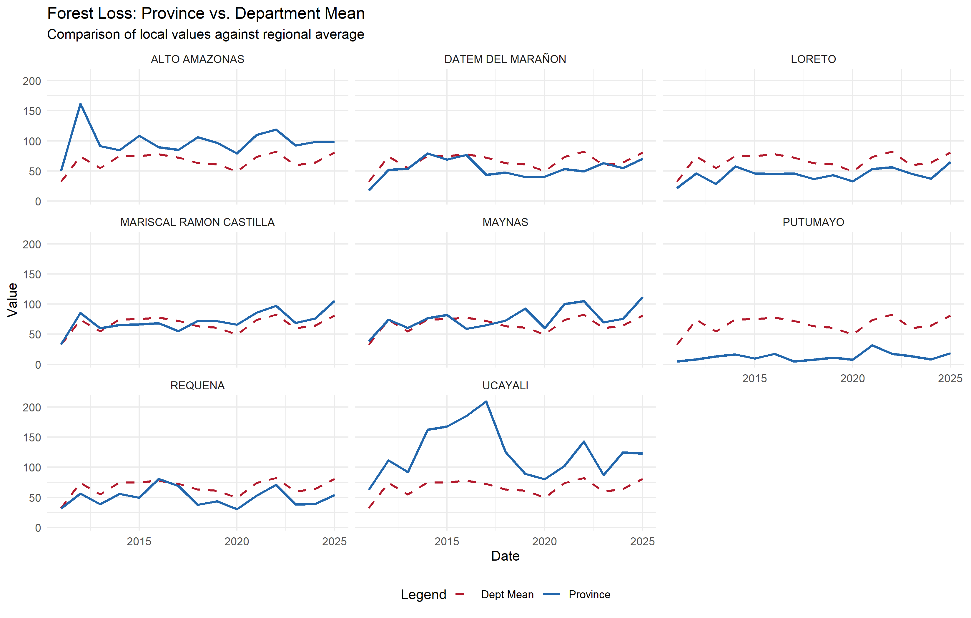
result_clean <- result |>
  mutate(
    year = format(as.Date(date), "%Y"),
    nombprov = toupper(trimws(as.character(nombprov)))
  )

q_vals <- quantile(
  result_clean$value,
  probs = c(0, 0.05, 0.25, 0.75, 0.95, 1),
  na.rm = TRUE
  )

q_labs <- c(
  paste0("< ", round(q_vals[2], 1)),
  paste0(round(q_vals[2:4], 1), " – ", round(q_vals[3:5], 1)),
  paste0("> ", round(q_vals[5], 1))
  )

pal <- c("#2166AC", "#67A9CF", "#F7F7F7", "#F4A582", "#B2182B")

result_clean %>%
  mutate(
    loss_cat = cut(
      value,
      breaks = q_vals,
      labels = q_labs,
      include.lowest = TRUE
      )
    ) %>%
  ggplot() +
  geom_sf(aes(fill = loss_cat), color = "#000000", linewidth = 0.15) +
  scale_fill_manual(
    name = "Forest Loss (km²)",
    values = setNames(pal,q_labs)
  ) +
  facet_wrap(~ year, ncol = 5) +
  labs(
    title = "Spatiotemporal Evolution of Tree Cover Loss by Province",
    subtitle = "Loreto, Peru (2011–2025)"
  ) +
  theme_minimal(base_size = 10)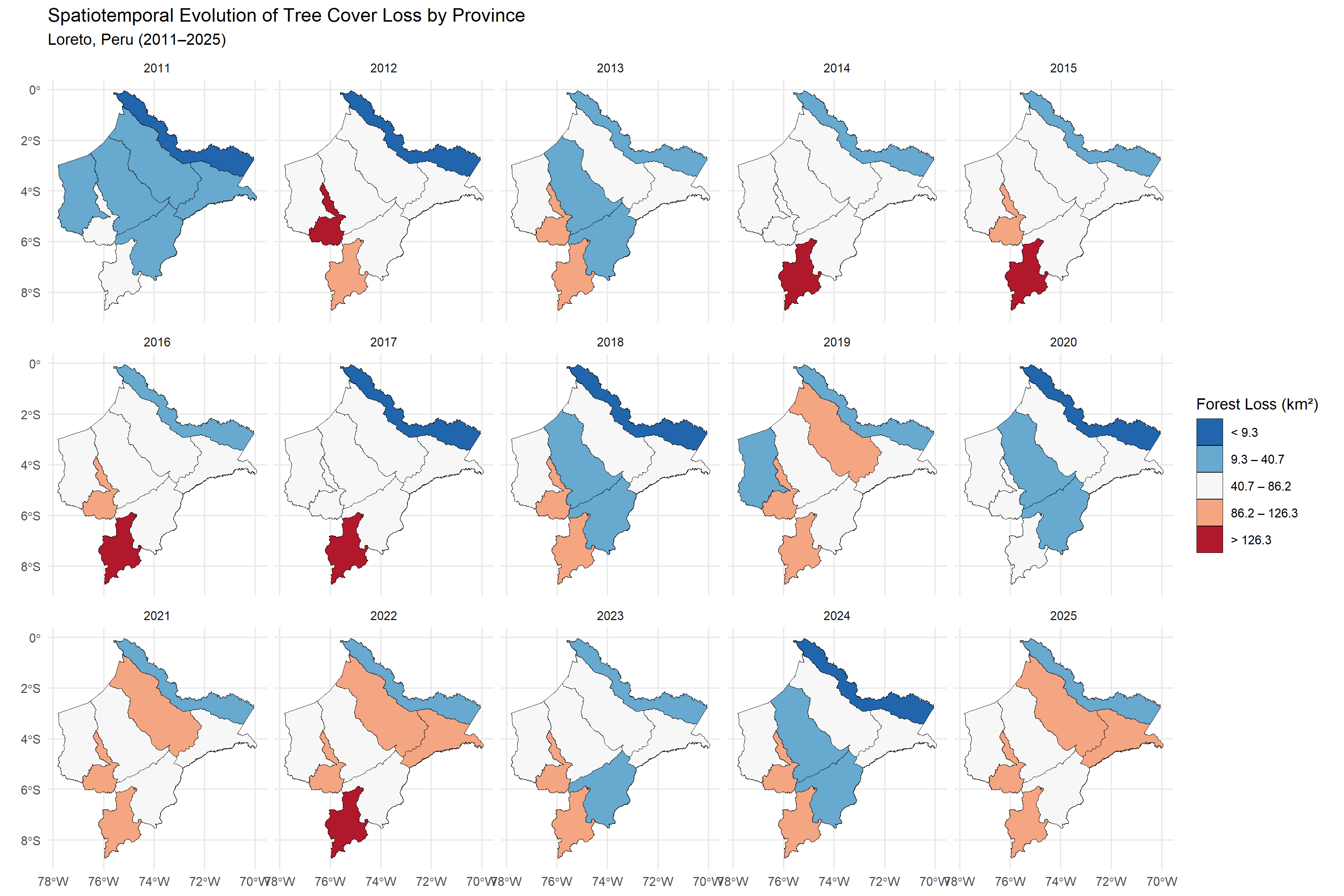
etp_ts <- provinces_loreto |>
  l4h_sebal_modis(
    from = "2005-01-01",
    to = "2022-12-31",
    by = "month"
  )
etp_base <- etp_ts |>
st_drop_geometry() |>
mutate(
nombprov = toupper(trimws(as.character(nombprov))),
month = as.numeric(format(as.Date(date), "%m"))
)
etp_loreto <- etp_base |>
group_by(month) |>
summarise(mean_loreto = mean(value, na.rm = TRUE), .groups = "drop")
etp_diff <- etp_base |>
group_by(nombprov, month) |>
summarise(mean_prov = mean(value, na.rm = TRUE), .groups = "drop") |>
inner_join(etp_loreto, by = "month") |>
mutate(
ymax_pos = pmax(mean_prov, mean_loreto),
ymin_neg = pmin(mean_prov, mean_loreto)
)
head(etp_diff)
#> # A tibble: 6 × 6
#> nombprov month mean_prov mean_loreto ymax_pos ymin_neg
#> <chr> <dbl> <dbl> <dbl> <dbl> <dbl>
#> 1 ALTO AMAZONAS 1 3165. 3106. 3165. 3106.
#> 2 ALTO AMAZONAS 2 3459. 3430. 3459. 3430.
#> 3 ALTO AMAZONAS 3 3264. 3192. 3264. 3192.
#> 4 ALTO AMAZONAS 4 3214. 3128. 3214. 3128.
#> 5 ALTO AMAZONAS 5 2912. 2915. 2915. 2912.
#> 6 ALTO AMAZONAS 6 2736. 2751. 2751. 2736.ggplot(etp_diff, aes(x = month)) +
geom_ribbon(
aes(ymin = mean_loreto, ymax = ymax_pos, fill = "Above Average"),
alpha = 0.6
) +
geom_ribbon(
aes(ymin = ymin_neg, ymax = mean_loreto, fill = "Below Average"),
alpha = 0.6
) +
geom_line(
aes(y = mean_loreto),
color = "#475569",
linetype = "dashed",
linewidth = 0.7
) +
geom_line(
aes(y = mean_prov),
color = "#0F172A",
linewidth = 0.8
) +
facet_wrap(~ nombprov, ncol = 4) +
scale_fill_manual(
name = "Regional Deviation",
values = c(
"Above Average" = "#EF4444",
"Below Average" = "#3B82F6"
)
) +
scale_x_continuous(
breaks = c(1, 4, 7, 10),
labels = c("Jan", "Apr", "Jul", "Oct")
) +
labs(
title = "Provincial ETP Differential vs. Regional Average",
subtitle = "Dashed line: Loreto Average | Red: ETP Excess | Blue: ETP Deficit",
x = NULL,
y = "Average ETP (mm)"
) +
theme_minimal(base_size = 8) +
theme(legend.position = "bottom")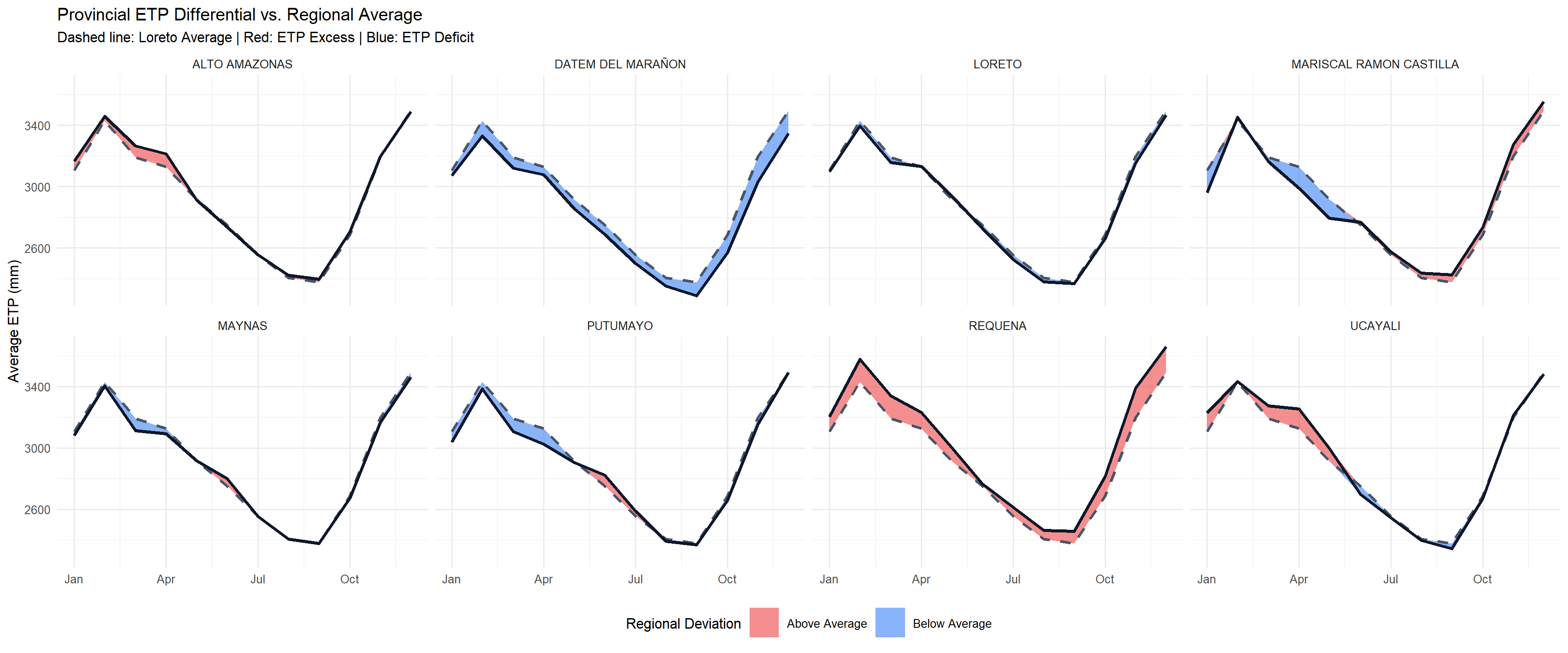
These binaries (installable software) and packages are in development.
They may not be fully stable and should be used with caution. We make no claims about them.
Health stats visible at Monitor.
