The hardware and bandwidth for this mirror is donated by dogado GmbH, the Webhosting and Full Service-Cloud Provider. Check out our Wordpress Tutorial.
If you wish to report a bug, or if you are interested in having us mirror your free-software or open-source project, please feel free to contact us at mirror[@]dogado.de.
![]()
![]()
Generate contour lines (isolines) and contour polygons (isobands) from regularly spaced grids containing elevation data. Package originally written by Claus Wilke and donated to r-lib in 2022.
Install the latest official release from CRAN via:
install.packages("isoband")Install the current development from github via:
# install.packages("pak")
pak::pak("r-lib/isoband")The two main workhorses of the package are the functions
isolines() and isobands(), respectively. They
return a list of isolines/isobands for each isolevel specified. Each
isoline/isoband consists of vectors of x and y coordinates, as well as a
vector of ids specifying which sets of coordinates should be connected.
This format can be handed directly to
grid.polyline()/grid.path() for drawing.
However, we can also convert the output to spatial features and draw
with ggplot2 (see below).
library(isoband)

m <- matrix(c(0, 0, 0, 0, 0,
              0, 1, 2, 1, 0,
              0, 1, 2, 0, 0,
              0, 1, 0, 1, 0,
              0, 0, 0, 0, 0), 5, 5, byrow = TRUE)

isolines(1:ncol(m), 1:nrow(m), m, 0.5)
#> $`0.5`
#> $`0.5`$x
#>  [1] 4.00 3.50 3.00 2.50 2.00 1.50 1.50 1.50 2.00 3.00 4.00 4.50 4.00 3.75 4.00
#> [16] 4.50 4.00
#>
#> $`0.5`$y
#>  [1] 4.50 4.00 3.75 4.00 4.50 4.00 3.00 2.00 1.50 1.25 1.50 2.00 2.50 3.00 3.50
#> [16] 4.00 4.50
#>
#> $`0.5`$id
#>  [1] 1 1 1 1 1 1 1 1 1 1 1 1 1 1 1 1 1
#>
#>
#> attr(,"class")
#> [1] "isolines" "iso"

isobands(1:ncol(m), 1:nrow(m), m, 0.5, 1.5)
#> $`0.5:1.5`
#> $`0.5:1.5`$x
#>  [1] 2.50 2.00 1.50 1.50 1.50 2.00 3.00 4.00 4.50 4.00 3.75 4.00 4.50 4.00 3.50
#> [16] 3.00 3.00 3.25 3.50 3.00 2.50 2.50
#>
#> $`0.5:1.5`$y
#>  [1] 4.00 4.50 4.00 3.00 2.00 1.50 1.25 1.50 2.00 2.50 3.00 3.50 4.00 4.50 4.00
#> [16] 3.75 3.25 3.00 2.00 1.75 2.00 3.00
#>
#> $`0.5:1.5`$id
#>  [1] 1 1 1 1 1 1 1 1 1 1 1 1 1 1 1 1 2 2 2 2 2 2
#>
#>
#> attr(,"class")
#> [1] "isobands" "iso"
The function plot_iso() is a convenience function for
debugging and testing.
plot_iso(m, 0.5, 1.5)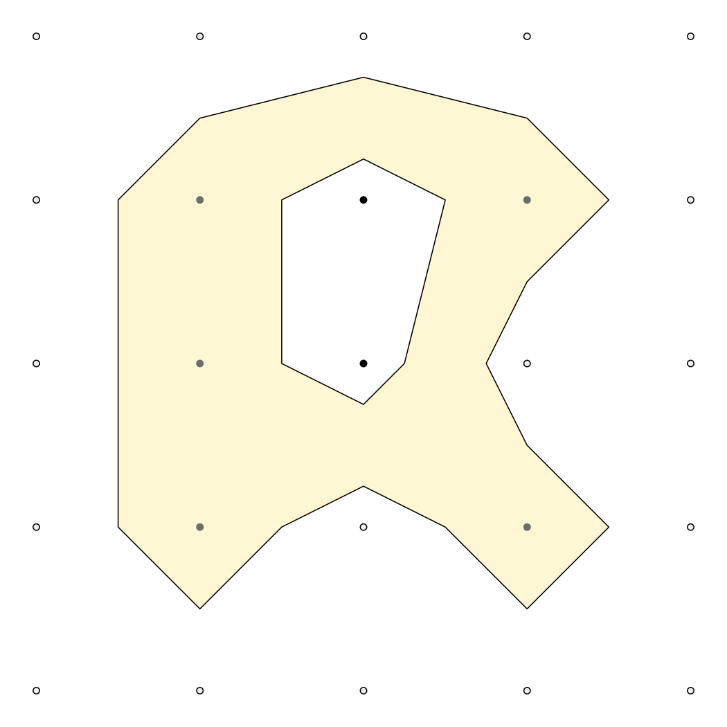
The isolining and isobanding algorithms have no problem with larger datasets. Let’s calculate isolines and isobands for the volcano dataset, convert to sf, and plot with ggplot2.
library(ggplot2)
suppressWarnings(library(sf))
#> Linking to GEOS 3.13.0, GDAL 3.8.5, PROJ 9.5.1; sf_use_s2() is TRUE

m <- volcano
b <- isobands((1:ncol(m))/(ncol(m)+1), (nrow(m):1)/(nrow(m)+1), m, 10*(9:19), 10*(10:20))
l <- isolines((1:ncol(m))/(ncol(m)+1), (nrow(m):1)/(nrow(m)+1), m, 10*(10:19))

bands <- iso_to_sfg(b)
data_bands <- st_sf(
  level = 1:length(bands),
  geometry = st_sfc(bands)
)
lines <- iso_to_sfg(l)
data_lines <- st_sf(
  level = 2:(length(lines)+1),
  geometry = st_sfc(lines)
)

ggplot() +
  geom_sf(data = data_bands, aes(fill = level), color = NA, alpha = 0.7) +
  geom_sf(data = data_lines, color = "black") +
  scale_fill_viridis_c(guide = "none") +
  coord_sf(expand = FALSE)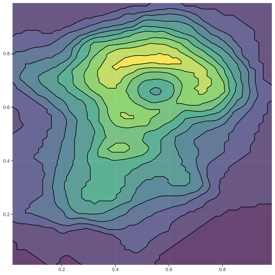
These binaries (installable software) and packages are in development.
They may not be fully stable and should be used with caution. We make no claims about them.
Health stats visible at Monitor.